MLR: Conditions

Prof. Eric Friedlander

Application Exercise

Complete the AE 15 - Inference for MLR (you may skip Exercise 5).

Once complete, Complete Exercises 0-6 of AE 16.

Topics

Inference for multiple linear regression
Checking model conditions

Computational setup

# load packages
library(tidyverse)

── Attaching core tidyverse packages ──────────────────────── tidyverse 2.0.0 ──
✔ dplyr     1.1.4     ✔ readr     2.1.5
✔ forcats   1.0.0     ✔ stringr   1.5.1
✔ ggplot2   3.5.1     ✔ tibble    3.2.1
✔ lubridate 1.9.3     ✔ tidyr     1.3.1
✔ purrr     1.0.2     
── Conflicts ────────────────────────────────────────── tidyverse_conflicts() ──
✖ dplyr::filter() masks stats::filter()
✖ dplyr::lag()    masks stats::lag()
ℹ Use the conflicted package (<http://conflicted.r-lib.org/>) to force all conflicts to become errors

library(broom)
library(mosaic)

Registered S3 method overwritten by 'mosaic':
  method                           from   
  fortify.SpatialPolygonsDataFrame ggplot2

The 'mosaic' package masks several functions from core packages in order to add 
additional features.  The original behavior of these functions should not be affected by this.

Attaching package: 'mosaic'

The following object is masked from 'package:Matrix':

    mean

The following objects are masked from 'package:dplyr':

    count, do, tally

The following object is masked from 'package:purrr':

    cross

The following object is masked from 'package:ggplot2':

    stat

The following objects are masked from 'package:stats':

    binom.test, cor, cor.test, cov, fivenum, IQR, median, prop.test,
    quantile, sd, t.test, var

The following objects are masked from 'package:base':

    max, mean, min, prod, range, sample, sum

library(mosaicData)
library(patchwork)
library(knitr)
library(kableExtra)


Attaching package: 'kableExtra'

The following object is masked from 'package:dplyr':

    group_rows

library(scales)


Attaching package: 'scales'

The following object is masked from 'package:mosaic':

    rescale

The following object is masked from 'package:purrr':

    discard

The following object is masked from 'package:readr':

    col_factor

library(GGally)

Registered S3 method overwritten by 'GGally':
  method from   
  +.gg   ggplot2

library(countdown)
library(rms)

Loading required package: Hmisc

Attaching package: 'Hmisc'

The following objects are masked from 'package:dplyr':

    src, summarize

The following objects are masked from 'package:base':

    format.pval, units

# set default theme and larger font size for ggplot2
ggplot2::theme_set(ggplot2::theme_minimal(base_size = 16))

Data: `rail_trail`

The Pioneer Valley Planning Commission (PVPC) collected data for ninety days from April 5, 2005 to November 15, 2005.
Data collectors set up a laser sensor, with breaks in the laser beam recording when a rail-trail user passed the data collection station.

Rows: 90 Columns: 7
── Column specification ────────────────────────────────────────────────────────
Delimiter: ","
chr (2): season, day_type
dbl (5): volume, hightemp, avgtemp, cloudcover, precip

ℹ Use `spec()` to retrieve the full column specification for this data.
ℹ Specify the column types or set `show_col_types = FALSE` to quiet this message.

Rows: 90
Columns: 7
$ volume     <dbl> 501, 419, 397, 385, 200, 375, 417, 629, 533, 547, 432, 418,…
$ hightemp   <dbl> 83, 73, 74, 95, 44, 69, 66, 66, 80, 79, 78, 65, 41, 59, 50,…
$ avgtemp    <dbl> 66.5, 61.0, 63.0, 78.0, 48.0, 61.5, 52.5, 52.0, 67.5, 62.0,…
$ season     <chr> "Summer", "Summer", "Spring", "Summer", "Spring", "Spring",…
$ cloudcover <dbl> 7.6, 6.3, 7.5, 2.6, 10.0, 6.6, 2.4, 0.0, 3.8, 4.1, 8.5, 7.2…
$ precip     <dbl> 0.00, 0.29, 0.32, 0.00, 0.14, 0.02, 0.00, 0.00, 0.00, 0.00,…
$ day_type   <chr> "Weekday", "Weekday", "Weekday", "Weekend", "Weekday", "Wee…

Source: Pioneer Valley Planning Commission via the mosaicData package.

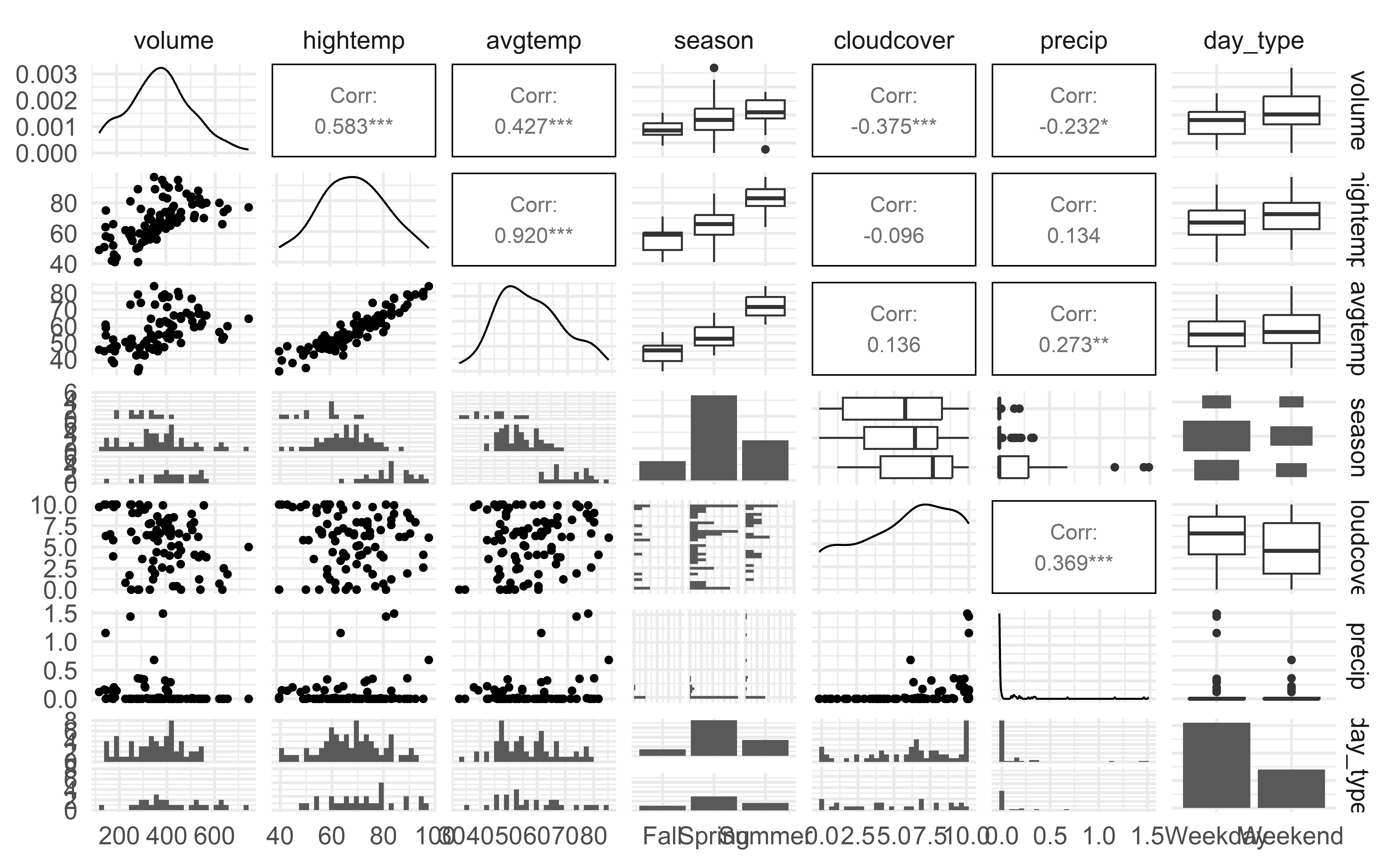
Visualizing the data

rail_trail |> ggpairs()

`stat_bin()` using `bins = 30`. Pick better value with `binwidth`.
`stat_bin()` using `bins = 30`. Pick better value with `binwidth`.
`stat_bin()` using `bins = 30`. Pick better value with `binwidth`.
`stat_bin()` using `bins = 30`. Pick better value with `binwidth`.
`stat_bin()` using `bins = 30`. Pick better value with `binwidth`.
`stat_bin()` using `bins = 30`. Pick better value with `binwidth`.
`stat_bin()` using `bins = 30`. Pick better value with `binwidth`.
`stat_bin()` using `bins = 30`. Pick better value with `binwidth`.
`stat_bin()` using `bins = 30`. Pick better value with `binwidth`.
`stat_bin()` using `bins = 30`. Pick better value with `binwidth`.

Conduct a hypothesis test for \(\beta_j\)

Multiple linear regression

rail_trail_fit <- lm(volume ~ avgtemp + hightemp, data = rail_trail)

tidy(rail_trail_fit) |> kable()

term	estimate	std.error	statistic	p.value
(Intercept)	1.667237	56.424299	0.0295482	0.9764951
avgtemp	-7.942489	2.346235	-3.3852060	0.0010689
hightemp	12.056606	2.041231	5.9065368	0.0000001

Multiple linear regression

The multiple linear regression model assumes \[Y|X_1, X_2, \ldots, X_p \sim N(\beta_0 + \beta_1 X_1 + \beta_2 X_2 + \dots + \beta_p X_p, \sigma_\epsilon^2)\]

For a given observation \((x_{i1}, x_{i2}, \ldots, x_{ip}, y_i)\), we can rewrite the previous statement as

\[y_i = \beta_0 + \beta_1 x_{i1} + \beta_2 x_{i2} + \dots + \beta_p x_{ip} + \epsilon_{i}, \hspace{10mm} \epsilon_i \sim N(0,\sigma_{\epsilon}^2)\]

Estimating \(\sigma_\epsilon\)

For a given observation \((x_{i1}, x_{i2}, \ldots,x_{ip}, y_i)\) the residual is \[ \begin{aligned} e_i &= y_{i} - \hat{y_i}\\ &= y_i - (\hat{\beta}_0 + \hat{\beta}_1 x_{i1} + \hat{\beta}_{2} x_{i2} + \dots + \hat{\beta}_p x_{ip}) \end{aligned} \]

The estimated value of the regression standard error , \(\sigma_{\epsilon}\), is

\[\hat{\sigma}_\epsilon = \sqrt{\frac{\sum_{i=1}^ne_i^2}{n-p-1}}\]

As with SLR, we use \(\hat{\sigma}_{\epsilon}\) to calculate \(SE_{\hat{\beta}_j}\), the standard error of each coefficient. See Matrix Form of Linear Regression for more detail.

MLR hypothesis test: avgtemp

Set hypotheses: \(H_0: \beta_{avgtemp} = 0\) vs. \(H_A: \beta_{avgtemp} \ne 0\), given hightemp is in the model

Calculate test statistic and p-value: The test statistic is \(t = -3.39\). The p-value is calculated using a \(t\) distribution with \[(n - p - 1) = 90 - 2 -1 = 87\] degrees of freedom. The p-value is \(\approx 0.0011\).
- Note that \(p\) counts all non-intercept \(\beta\)’s

State the conclusion: The p-value is small, so we reject \(H_0\). The data provides convincing evidence that a avgtemp is a useful predictor in a model that already contains rail_trail hightemp as a predictor for the rail_trail volume.

MLR hypothesis test: interaction terms

Framework: Same as previous slide except use \(\beta\) of interaction term
\(p\) (the number of predictors) should include the interaction term
Conclusion: tells you whether interaction term is a useful predictor
Warning: if \(X_1\) and \(X_2\) have an interaction term, don’t try to interpret their individual p-values… if interaction term is significant, then both variables are important

Confidence interval for \(\beta_j\)

The \(C\%\) confidence interval for \(\beta_j\) \[\hat{\beta}_j \pm t^* SE(\hat{\beta}_j)\] where \(t^*\) follows a \(t\) distribution with \(n - p - 1\) degrees of freedom.
Generically: We are \(C\%\) confident that the interval LB to UB contains the population coefficient of \(x_j\).
In context: We are \(C\%\) confident that for every one unit increase in \(x_j\), we expect \(y\) to change by LB to UB units, holding all else constant.

Confidence interval for \(\beta_j\)

term	estimate	std.error	statistic	p.value	conf.low	conf.high
(Intercept)	1.67	56.42	0.03	0.98	-110.48	113.82
avgtemp	-7.94	2.35	-3.39	0.00	-12.61	-3.28
hightemp	12.06	2.04	5.91	0.00	8.00	16.11

Inference pitfalls

Large sample sizes

Caution

If the sample size is large enough, the test will likely result in rejecting \(H_0: \beta_j = 0\) even \(x_j\) has a very small effect on \(y\).

Consider the practical significance of the result not just the statistical significance.
Instead of saying statistically significant say statistically detectable
Use confidence intervals to draw conclusions instead of relying only on p-values.

Small sample sizes

Caution

If the sample size is small, there may not be enough evidence to reject \(H_0: \beta_j=0\).

When you fail to reject the null hypothesis, DON’T immediately conclude that the variable has no association with the response.
There may be a linear association that is just not strong enough to detect given your data, or there may be a non-linear association.

Conditions for inference

Model conditions

Our model conditions are the same as they were with SLR:

Linearity: There is a linear relationship between the response and predictor variables.
Constant Variance: The variability about the least squares line is generally constant.
Normality: The distribution of the residuals is approximately normal.
Independence: The residuals are independent from each other.

Checking Linearity

Look at a plot of the residuals vs. predicted values
Look at a plot of the residuals vs. each predictor
- Use scatter plots for quantitative and boxplots of categorical predictors
Linearity is met if there is no discernible pattern in each of these plots

Complete Exercises 7-10

Fitting the Full Model

full_model <- lm(volume ~ . , data = rail_trail)
full_model |> tidy() |>  kable()

term	estimate	std.error	statistic	p.value
(Intercept)	17.622161	76.582860	0.2301058	0.8185826
hightemp	7.070528	2.420523	2.9210743	0.0045045
avgtemp	-2.036685	3.142113	-0.6481896	0.5186733
seasonSpring	35.914983	32.992762	1.0885716	0.2795319
seasonSummer	24.153571	52.810486	0.4573632	0.6486195
cloudcover	-7.251776	3.843071	-1.8869743	0.0627025
precip	-95.696525	42.573359	-2.2478030	0.0272735
day_typeWeekend	35.903750	22.429056	1.6007696	0.1132738

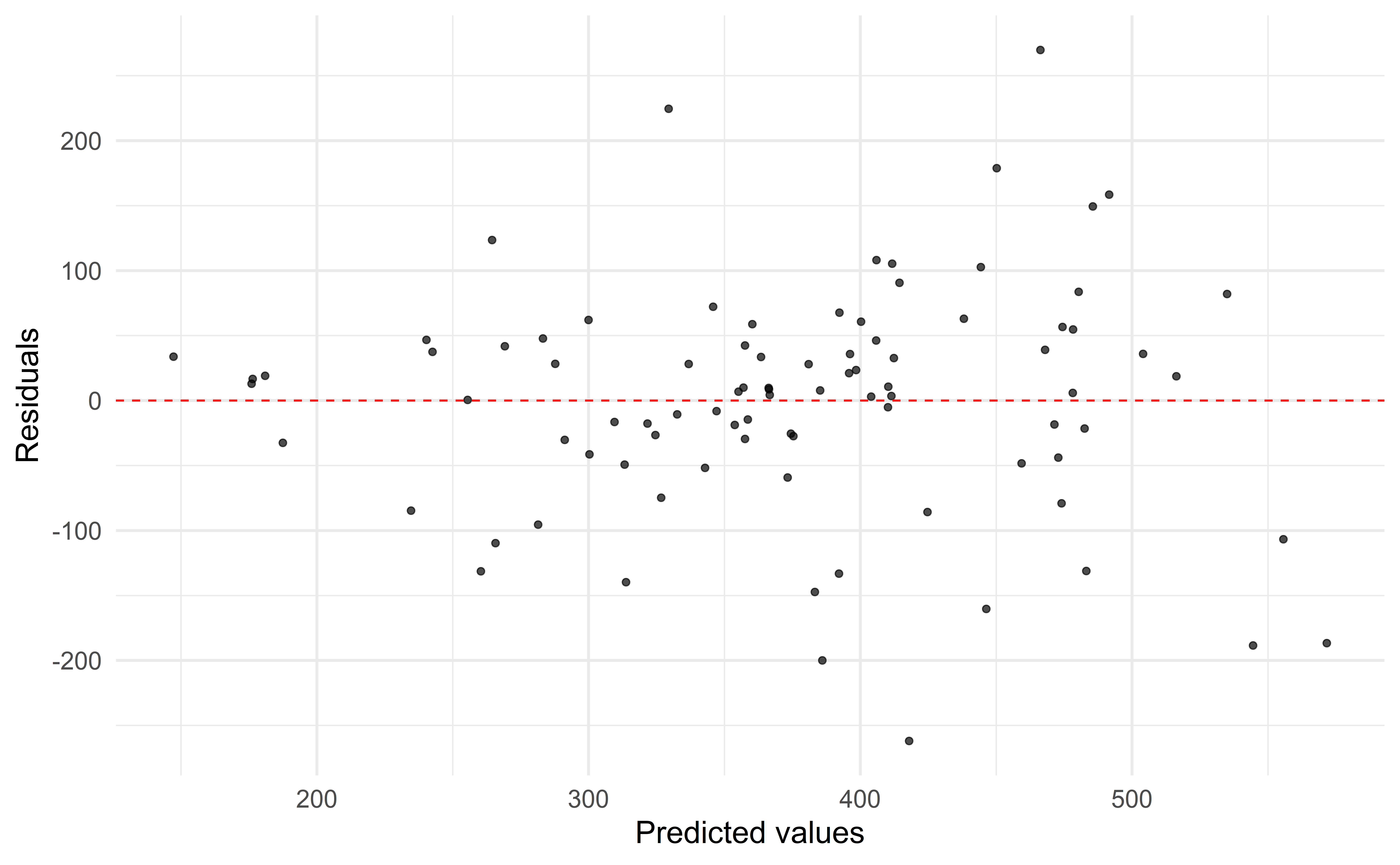
Residuals vs. predicted values

Does the constant variance condition appear to be satisfied?

Checking constant variance

The vertical spread of the residuals is not constant across the plot.
The constant variance condition is not satisfied.

Given this conclusion, what might be a next step in the analysis?

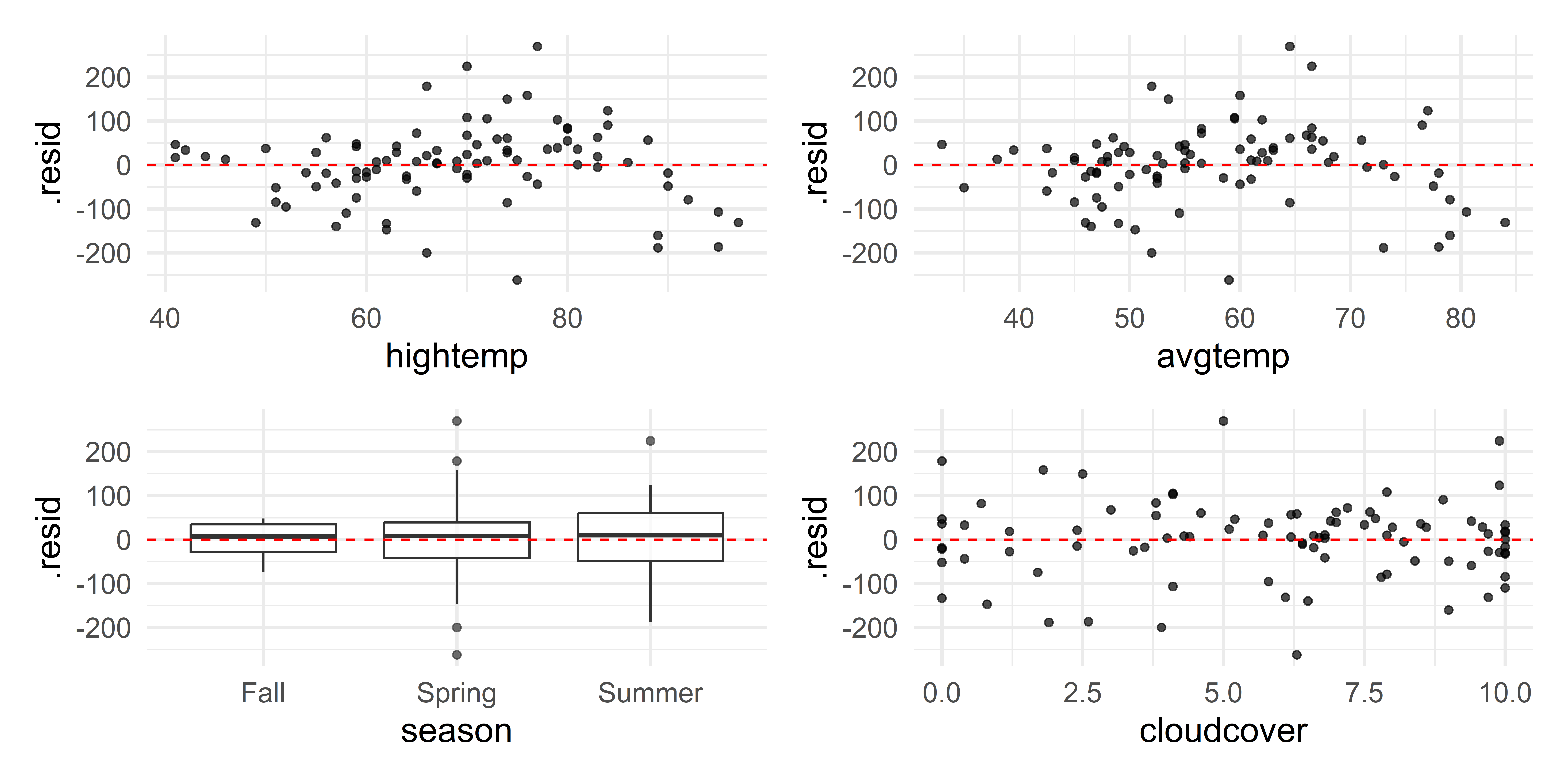
Residuals vs. each predictor

Checking linearity

The plot of the residuals vs. predicted values looked OK
The plots of residuals vs. hightemp and avgtemp appear to have a parabolic pattern.
The linearity condition does not appear to be satisfied given these plots.

Given this conclusion, what might be a next step in the analysis?

Complete Exercises 11-12.

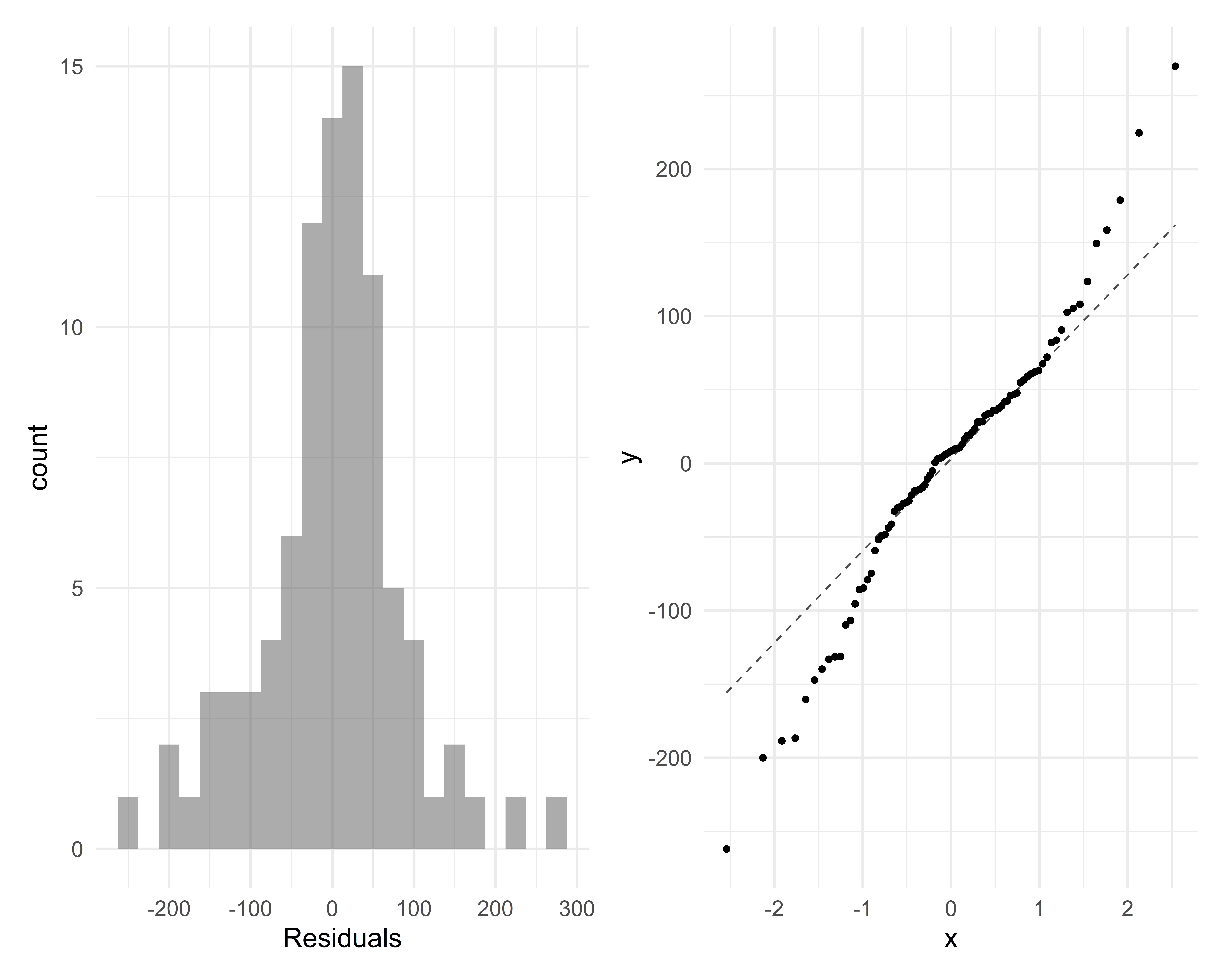
Checking normality

The distribution of the residuals is approximately unimodal and symmetric but the qqplot shows that tails are too heavy, so the normality condition is likely not satisfied. The sample size 90 is sufficiently large to relax this condition.

Checking independence

We can often check the independence condition based on the context of the data and how the observations were collected.
If the data were collected in a particular order, examine a scatter plot of the residuals versus order in which the data were collected.
If there is a grouping variable lurking in the background, check the residuals based on that grouping variable.

Recap

Inference for individual predictors
- Hypothesis testing: same as SLR but add if all other terms are in the model
- Confidence intervals: same as SLR but add holding all other variables in the model constant
Conditions: Same as for SLR
- For linearity, also check fitter values vs. each predictor

MLR: Conditions

Application Exercise

Topics

Computational setup

Data: rail_trail

Visualizing the data

Conduct a hypothesis test for \(\beta_j\)

Multiple linear regression

Multiple linear regression

Estimating \(\sigma_\epsilon\)

MLR hypothesis test: avgtemp

MLR hypothesis test: interaction terms

Confidence interval for \(\beta_j\)

Confidence interval for \(\beta_j\)

Confidence interval for \(\beta_j\)

Inference pitfalls

Large sample sizes

Small sample sizes

Conditions for inference

Model conditions

Checking Linearity

Fitting the Full Model

Residuals vs. predicted values

Checking constant variance

Residuals vs. each predictor

Checking linearity

Checking normality

Checking independence

Recap

Data: `rail_trail`