# load packages
library(tidyverse)
library(broom)
library(mosaic)
library(Stat2Data)
library(patchwork)
library(knitr)
library(kableExtra)
library(scales)
library(GGally)
library(countdown)
library(rms)
library(coursekata)

# set default theme and larger font size for ggplot2
ggplot2::theme_set(ggplot2::theme_minimal(base_size = 16))MLR: Inference
Application Exercise
📋 AE 15 - Inference for MLR
- Complete Exercises 0-1
Topics
- Inference for multiple linear regression
- Effect Size and Power
Computational setup
Data: Tadpoles
Biologists wondered whether tadpoles can adjust the relative length of their intestines if they are exposed to a fungus called Batrachochytrium dendrobatidis (Bd).
Rows: 27
Columns: 4
$ Treatment       <fct> Bd, Bd, Bd, Bd, Bd, Bd, Bd, Bd, Bd, Bd, Bd, Bd, Bd, Bd…
$ Body            <dbl> 20.28, 19.75, 19.28, 17.81, 20.79, 16.99, 18.12, 16.95…
$ GutLength       <dbl> 191.40, 142.92, 169.81, 152.18, 171.33, 153.92, 181.08…
$ MouthpartDamage <dbl> 0.679, 0.607, 0.750, 0.821, 0.696, 0.571, 0.571, 0.571…
Source: Stat2Data.
Conduct a hypothesis test for \(\beta_j\)
Review: Simple linear regression (SLR)
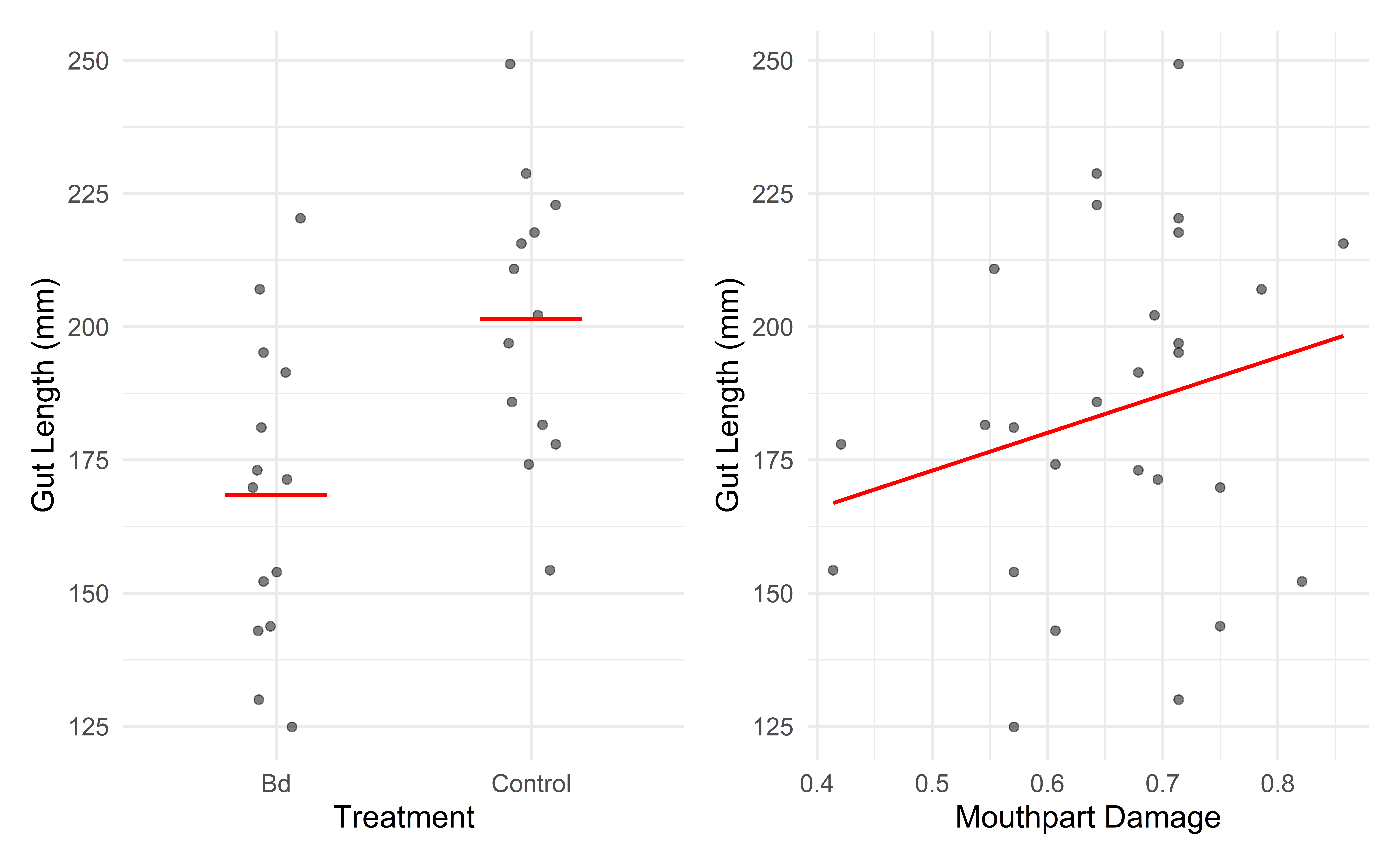
p1 <- gf_jitter(GutLength ~ Treatment, data = Tadpoles, alpha = 0.5, height = 0, width = 0.1) |>
  gf_model(lm(GutLength ~ Treatment, data = Tadpoles), color = "red") |>
  gf_labs(x = "Treatment", y = "Gut Length (mm)")
p2 <- gf_point(GutLength ~ MouthpartDamage, data = Tadpoles, alpha = 0.5) |>
  gf_model(lm(GutLength ~ MouthpartDamage, data = Tadpoles), color = "red") |>
  gf_labs(x = "Mouthpart Damage", y = "Gut Length (mm)")
p1 + p2
SLR model summary
Code
| term | estimate | std.error | statistic | p.value |
|---|---|---|---|---|
| (Intercept) | 168.34714 | 7.357157 | 22.882092 | 0.0000000 |
| TreatmentControl | 33.02824 | 10.602792 | 3.115051 | 0.0045722 |
| term | estimate | std.error | statistic | p.value |
|---|---|---|---|---|
| (Intercept) | 137.57782 | 39.07066 | 3.521256 | 0.0016738 |
| MouthpartDamage | 70.85005 | 58.59173 | 1.209216 | 0.2378918 |
SLR hypothesis test
- Set hypotheses: \(H_0: \beta_1 = 0\) vs. \(H_A: \beta_1 \ne 0\)
Calculate test statistic and p-value . . .
State the conclusion
Multiple linear regression
- Discussion: How should we handle our confounding variables?
Complete Exercise 2.
Multiple linear regression
The multiple linear regression model assumes \[Y|X_1, X_2, \ldots, X_p \sim N(\beta_0 + \beta_1 X_1 + \beta_2 X_2 + \dots + \beta_p X_p, \sigma_\epsilon^2)\]
For a given observation \((x_{i1}, x_{i2}, \ldots, x_{ip}, y_i)\), we can rewrite the previous statement as
\[y_i = \beta_0 + \beta_1 x_{i1} + \beta_2 x_{i2} + \dots + \beta_p x_{ip} + \epsilon_{i}, \hspace{10mm} \epsilon_i \sim N(0,\sigma_{\epsilon}^2)\]
Estimating \(\sigma_\epsilon\)
For a given observation \((x_{i1}, x_{i2}, \ldots,x_{ip}, y_i)\) the residual is \[ \begin{aligned} e_i &= y_{i} - \hat{y_i}\\ &= y_i - (\hat{\beta}_0 + \hat{\beta}_1 x_{i1} + \hat{\beta}_{2} x_{i2} + \dots + \hat{\beta}_p x_{ip}) \end{aligned} \]
The estimated value of the regression standard error , \(\sigma_{\epsilon}\), is
\[\hat{\sigma}_\epsilon = \sqrt{\frac{\sum_{i=1}^ne_i^2}{n-p-1}}\]
As with SLR, we use \(\hat{\sigma}_{\epsilon}\) to calculate \(SE_{\hat{\beta}_j}\), the standard error of each coefficient. See Matrix Form of Linear Regression for more detail.
MLR Model
MLR hypothesis test: treatment
- Set hypotheses: \(H_0: \beta_{trmt} = 0\) vs. \(H_A: \beta_{trmt} \ne 0\), given other
Bodyis in the model
Calculate test statistic and p-value: The test statistic is \(t = 1.48\). The p-value is calculated using a \(t\) distribution with \[(n - p - 1) = 27-2-1 = 24\] degrees of freedom. The p-value is \(\approx 0.153\).
- Note that \(p\) counts all non-intercept \(\beta\)’s
- State the conclusion: The p-value provides no evidence in favor of the alternative, so we fail to reject \(H_0\). The data does not provide evidence that a exposure to the Bd fungus is a useful predictor in a model that already contains body length as a predictor of gut length (could also say when controlling for body length).
MLR hypothesis test: interaction terms
- Framework: Same as previous slide except use \(\beta\) of interaction term
- \(p\) (the number of predictors) should include the interaction term
- Conclusion: tells you whether interaction term is a useful predictor
- Warning: if \(X_1\) and \(X_2\) have an interaction term, don’t try to interpret their individual p-values… if interaction term is significant, then both variables are important
Complete Exercises 3.
Effect Size and Power
Overview
- Effect Size:
- General Idea: how big is your parameter compared to the variability of your data
- Why is it important: if parameter has small effect size, it may not be a useful parameter to include. However, what effect size is useful depends on your problem
- In practice: many formal ways of determining effects size which we won’t talk about
- Statistical Power: the ability of a hypothesis test to detect a given effect size
- more data = more power
- tons of data = tons of power
- In practice: think about how what effect size you’d like to be able to detect and design your study to collect enough data to do so
Effect Size
- A few measures of effect size
- Cohen’s \(d\) (for when you have two groups: e.g. treament vs. control)
- \(R^2\) (for when you have continuous predictors)
- When evaluating effect size, consider practical significance not just statistical significance
- Effect size DOESN’T depend on sample size (other than sampling variability)
- Statistical significance DOES depend on sample size
Power
- Power: probability of correctly rejecting null hypothesis given a certain effect size
- Power depends on:
- Effect size
- Sample size
- Significance level (\(\alpha\))
- Variability in the data
- In practice: decide on a minimum effect size you want to be able to detect, then design your study to have enough power to detect that effect size
Power Analysis using Simulation
Power Analysis using Simulation I
set.seed(2025)
sample_size <- 50
lm(GutLength ~ Treatment + Body, data = resample(Tadpoles, sample_size)) |>
  tidy()
# A tibble: 3 × 5
term estimate std.error statistic p.value
<chr> <dbl> <dbl> <dbl> <dbl>
1 (Intercept) 35.1 42.3 0.831 0.410
2 TreatmentControl 16.9 8.04 2.10 0.0407
3 Body 7.24 2.18 3.32 0.00176Power Analysis using Simulation II
Power Analysis using Simulation III
sample_size <- 50
do(10) * lm(GutLength ~ Treatment + Body, data = resample(Tadpoles, sample_size)) |>
  tidy()
# A tibble: 30 × 7
term estimate std.error statistic p.value .row .index
<chr> <dbl> <dbl> <dbl> <dbl> <int> <dbl>
1 (Intercept) 24.6 35.1 0.700 0.487 1 1
2 TreatmentControl 16.8 8.62 1.94 0.0580 2 1
3 Body 7.59 1.85 4.10 0.000165 3 1
4 (Intercept) -15.8 34.4 -0.458 0.649 1 2
5 TreatmentControl -0.741 8.80 -0.0842 0.933 2 2
6 Body 10.1 1.83 5.51 0.00000146 3 2
7 (Intercept) 21.5 43.6 0.493 0.624 1 3
8 TreatmentControl 30.1 8.29 3.63 0.000700 2 3
9 Body 7.16 2.33 3.07 0.00357 3 3
10 (Intercept) 27.1 36.9 0.734 0.467 1 4
# ℹ 20 more rowsPower Analysis using Simulation IV
sample_size <- 50
do(10) * lm(GutLength ~ Treatment + Body, data = resample(Tadpoles, sample_size)) |>
  tidy() |>
  filter(term == "TreatmentControl")
# A tibble: 10 × 7
term estimate std.error statistic p.value .row .index
<chr> <dbl> <dbl> <dbl> <dbl> <int> <dbl>
1 TreatmentControl 10.5 8.31 1.26 0.213 1 1
2 TreatmentControl 9.60 6.03 1.59 0.118 1 2
3 TreatmentControl 11.6 8.20 1.41 0.164 1 3
4 TreatmentControl 16.5 7.24 2.27 0.0276 1 4
5 TreatmentControl 22.3 7.36 3.03 0.00399 1 5
6 TreatmentControl 2.45 6.63 0.369 0.714 1 6
7 TreatmentControl 17.2 8.38 2.06 0.0454 1 7
8 TreatmentControl 20.8 8.31 2.51 0.0158 1 8
9 TreatmentControl 24.1 7.98 3.02 0.00405 1 9
10 TreatmentControl 19.4 6.76 2.88 0.00602 1 10Power Analysis using Simulation IV
sample_size <- 50
samp_dist <- do(1000) * lm(GutLength ~ Treatment + Body, data = resample(Tadpoles, sample_size)) |>
  tidy() |>
  filter(term == "TreatmentControl")

tally(samp_dist$p.value < 0.05, format = "proportion")
X
TRUE FALSE
0.56 0.44 The power for a sample of size 50 if we assume the same effect size as in our data is approximately 0.56.
Complete Exercise 4.
Confidence interval for \(\beta_j\)
Confidence interval for \(\beta_j\)
The \(C\%\) confidence interval for \(\beta_j\) \[\hat{\beta}_j \pm t^* SE(\hat{\beta}_j)\] where \(t^*\) follows a \(t\) distribution with \(n - p - 1\) degrees of freedom.
Generically: We are \(C\%\) confident that the interval LB to UB contains the population coefficient of \(x_j\).
In context: We are \(C\%\) confident that for every one unit increase in \(x_j\), we expect \(y\) to change by LB to UB units, holding all else constant.
Complete Exercise 5.
Inference pitfalls
Large sample sizes
Caution
If the sample size is large enough, the test will likely result in rejecting \(H_0: \beta_j = 0\) even \(x_j\) has a very small effect on \(y\).
Consider the practical significance of the result not just the statistical significance.
Instead of saying statistically significant say statistically detectable
Use confidence intervals to draw conclusions instead of relying only on p-values.
Small sample sizes
Caution
If the sample size is small, there may not be enough evidence to reject \(H_0: \beta_j=0\).
When you fail to reject the null hypothesis, DON’T immediately conclude that the variable has no association with the response.
There may be a linear association that is just not strong enough to detect given your data, or there may be a non-linear association.
Recap
- Inference for individual predictors
- Hypothesis testing: same as SLR but add if all other terms are in the model
- Confidence intervals: same as SLR but add holding all other variables in the model constant
- Effect size and power
- Effect size: how big is your parameter compared to variability of data
- Power: ability to detect a given effect size
