# load packages
library(tidyverse)
library(broom)
library(mosaic)
library(ISLR2)
library(patchwork)
library(knitr)
library(coursekata)
library(kableExtra)
library(scales)

# set default theme and larger font size for ggplot2
ggplot2::theme_set(ggplot2::theme_minimal(base_size = 16))

# Create new variable

Credit <- Credit |>
mutate(Has_Balance = factor(ifelse(Balance == 0, "No", "Yes")))Categorical Predictors
Outcome: Limit
| min | Q1 | median | Q3 | max | mean | sd | n | missing | |
|---|---|---|---|---|---|---|---|---|---|
| 855 | 3088 | 4622.5 | 5872.75 | 13913 | 4735.6 | 2308.199 | 400 | 0 |
Predictors
Code
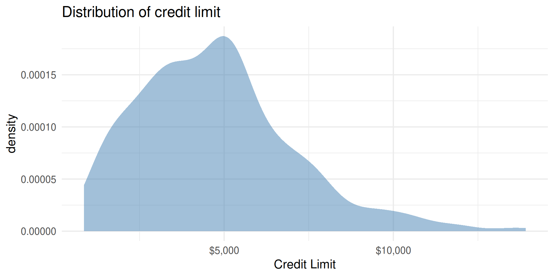
p1 <- Credit |>
  gf_density(~Limit, fill = "steelblue") |>
  gf_labs(title = "Distribution of credit limit",
          x = "Credit Limit")|>
    gf_refine(scale_x_continuous(labels = dollar_format()))

p2 <- Credit |>
  gf_histogram(~Rating, binwidth = 50) |>
  gf_labs(title = "",
       x = "Credit Rating")

p3 <- Credit |>
  gf_histogram(~Cards, binwidth = 1) |>
  gf_labs(title = "",
       x = "Number of Credit Cards")

p4 <- Credit |>
  gf_bar(~Has_Balance)|>
  gf_labs(title = "",
       x = "Has a Credit Card Balance")

(p1 + p2) / (p3 + p4)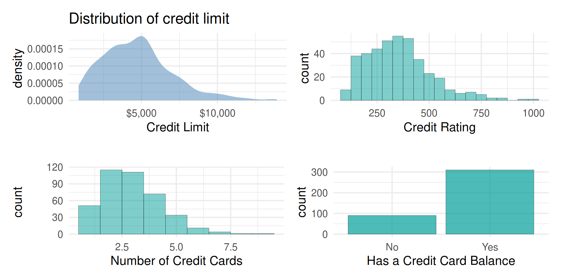
Outcome vs. predictors
Interpreting Categorical Predictors
| term | estimate | std.error | statistic | p.value |
|---|---|---|---|---|
| (Intercept) | 2152.722 | 194.211 | 11.084 | 0 |
| Has_BalanceYes | 3332.746 | 220.609 | 15.107 | 0 |
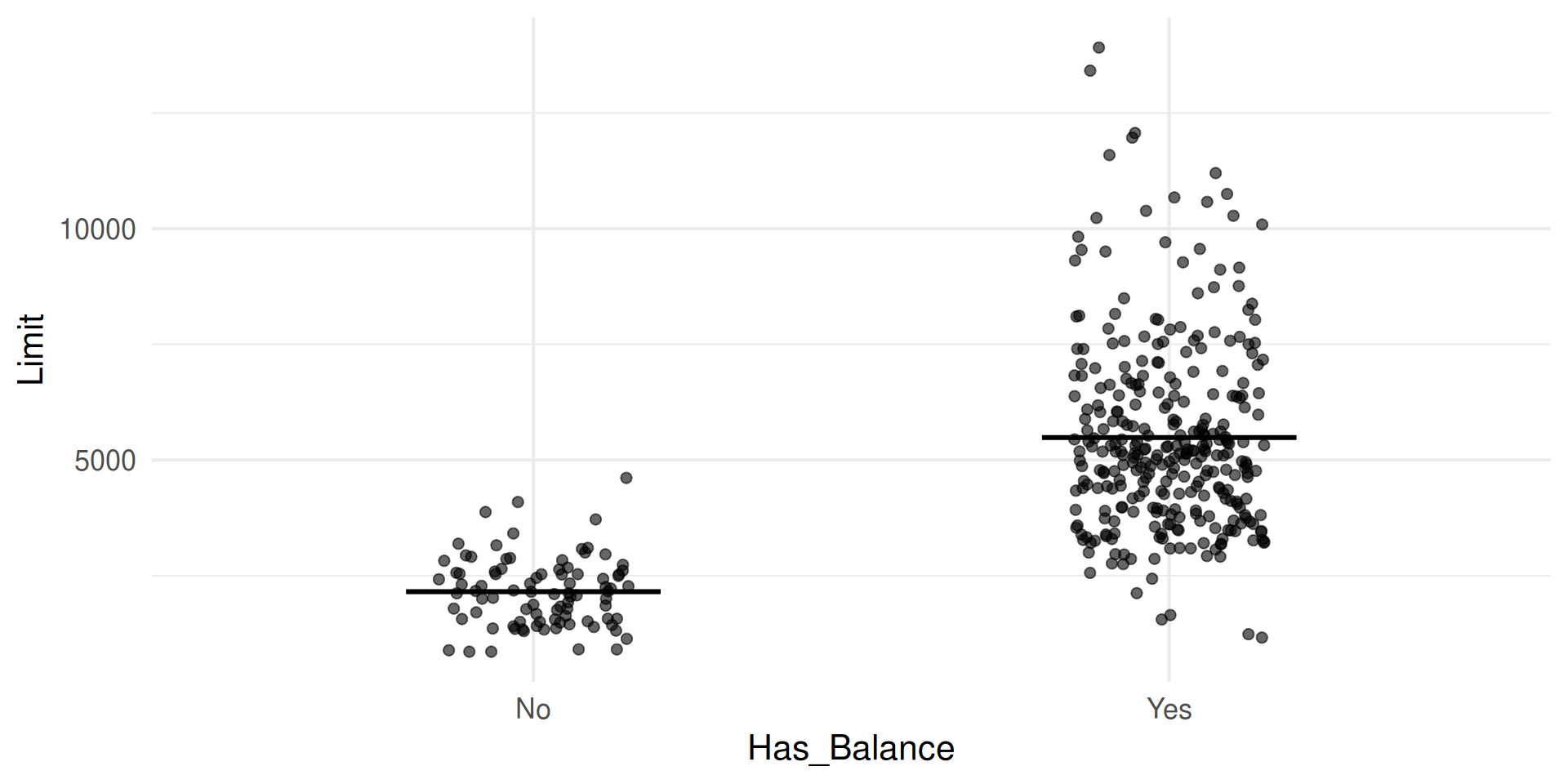
- Where do we see each of the estimates in the plot?
- Where do we see the values we’d predict in the plot?
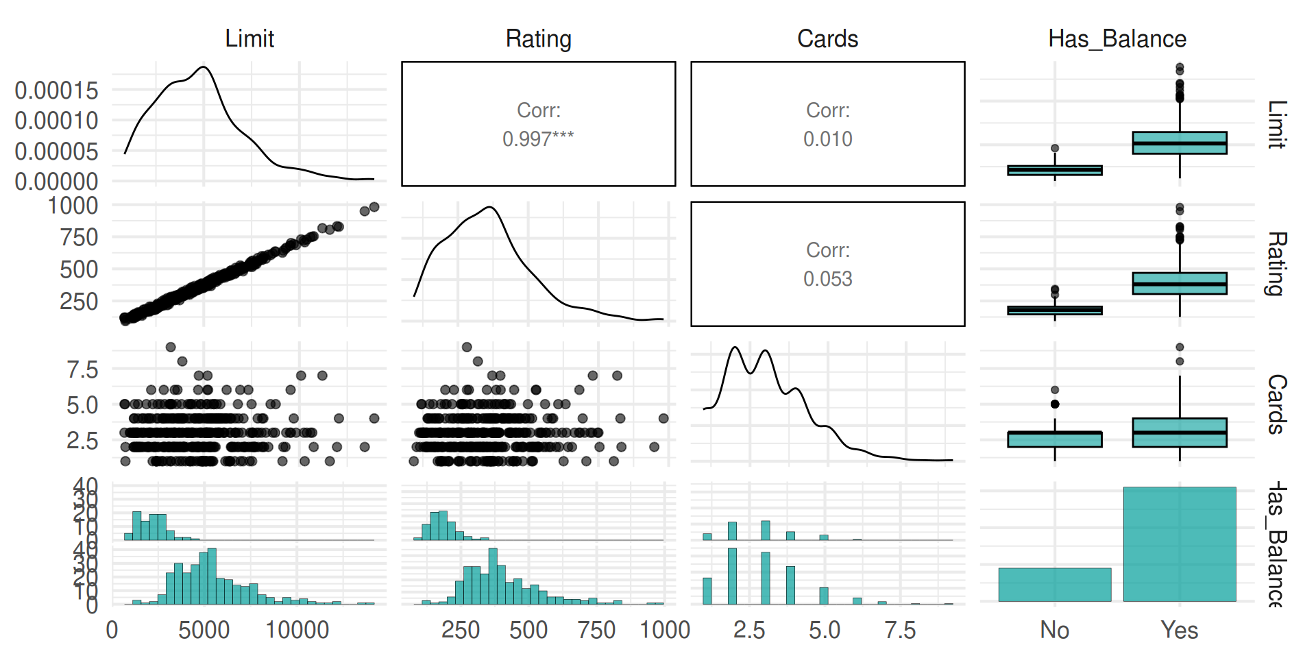
- (Trick Question) Are
Has_BalanceandLimitcorrelated? - On the board. Write down the dummy coding for an observation from each level in your chosen categorical variable.
Complete Exercises 2-4.
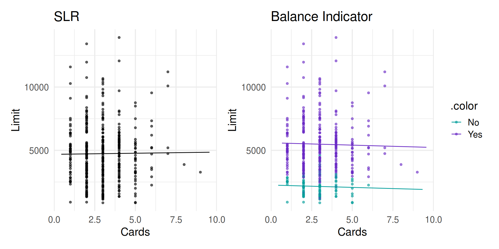
Credit Limit vs. Cards: parallel slopes
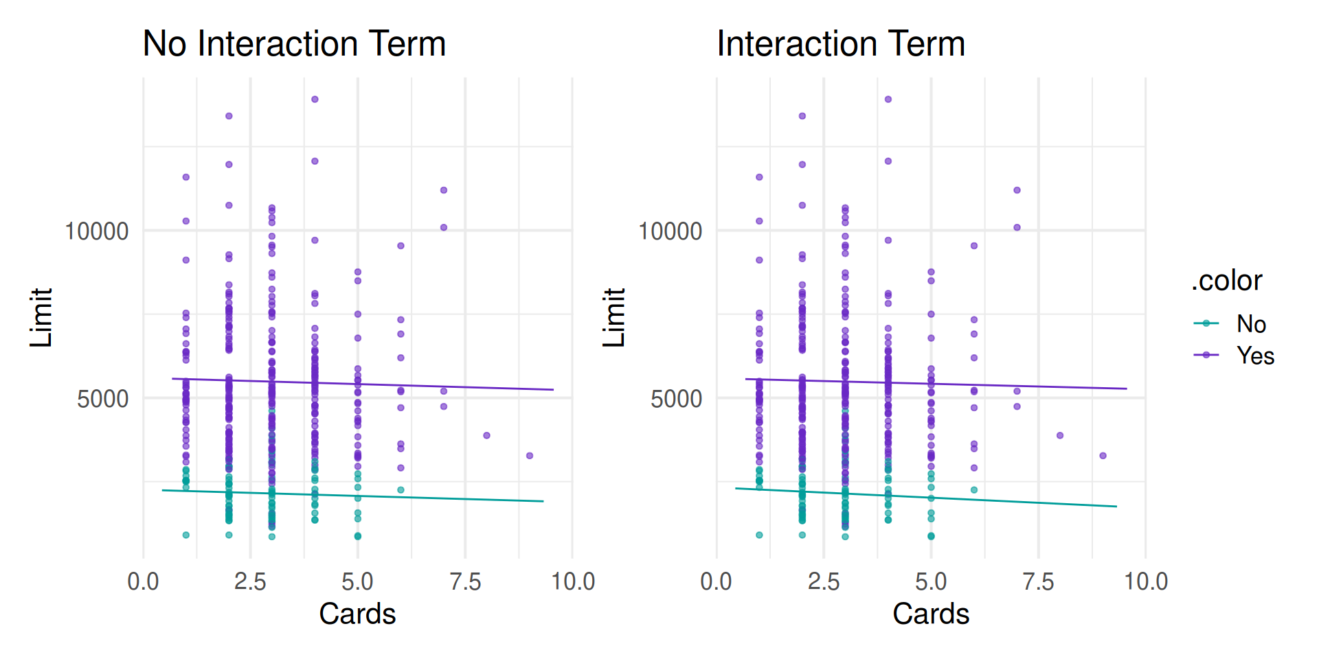
Interest rate vs. cards: interaction term
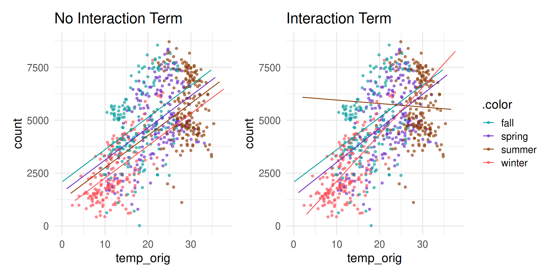
Bike Rentals vs. Temperature: interaction term