Multiple linear regression (MLR)

Prof. Eric Friedlander

Application Exercise

📋 AE 13 - Multiple Linear Regression and Categorical Predictors

Complete Exercise 0-3.

Computational setup

# load packages
library(tidyverse)
library(broom)
library(mosaic)
library(ISLR2)
library(patchwork)
library(knitr)
library(coursekata)
library(kableExtra)
library(scales)

# set default theme and larger font size for ggplot2
ggplot2::theme_set(ggplot2::theme_minimal(base_size = 16))

# Create new variable

Credit <- Credit |> 
  mutate(Has_Balance = factor(ifelse(Balance == 0, "No", "Yes")))

Considering multiple variables

Data: Credit Cards

The data is from the Credit data set in the ISLR2 R package. It is a simulated data set of 400 credit card customers.

Rows: 400
Columns: 12
$ Income      <dbl> 14.891, 106.025, 104.593, 148.924, 55.882, 80.180, 20.996,…
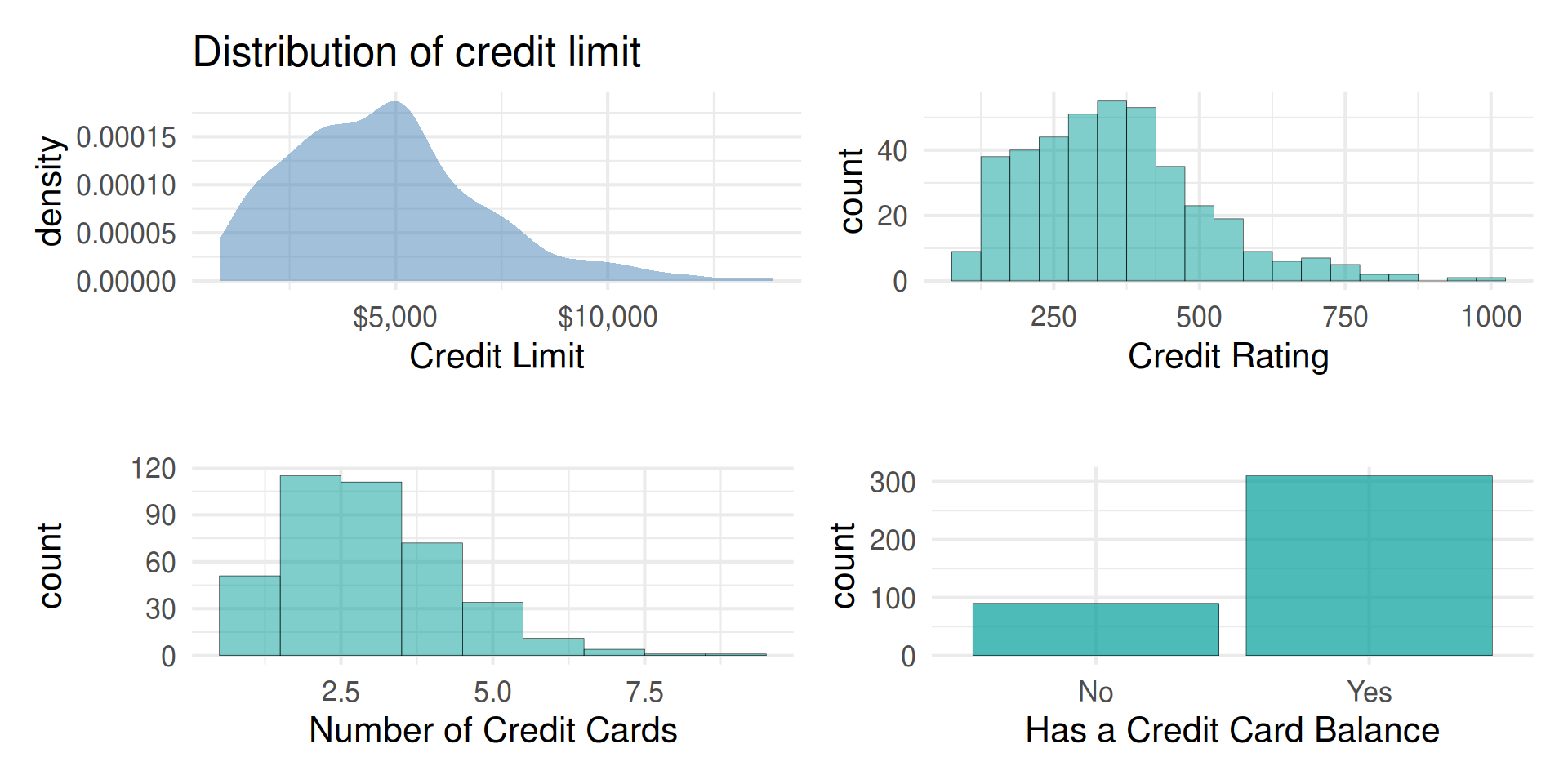
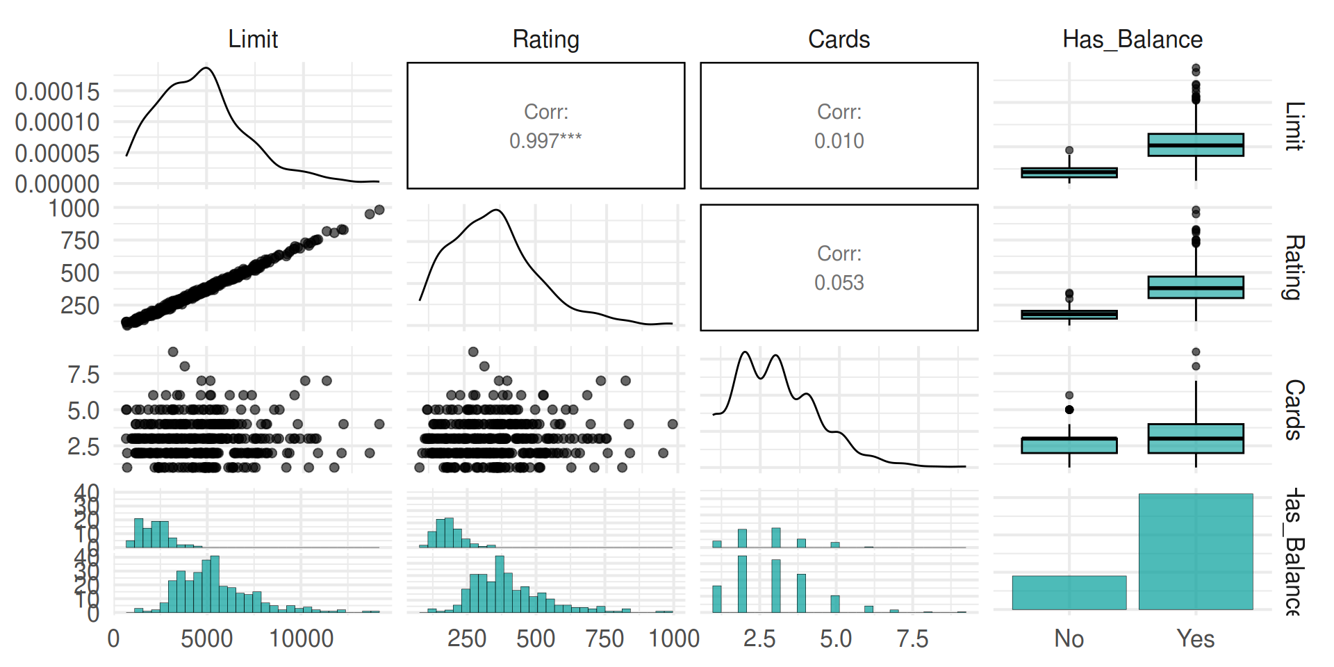
$ Limit       <dbl> 3606, 6645, 7075, 9504, 4897, 8047, 3388, 7114, 3300, 6819…
$ Rating      <dbl> 283, 483, 514, 681, 357, 569, 259, 512, 266, 491, 589, 138…
$ Cards       <dbl> 2, 3, 4, 3, 2, 4, 2, 2, 5, 3, 4, 3, 1, 1, 2, 3, 3, 3, 1, 2…
$ Age         <dbl> 34, 82, 71, 36, 68, 77, 37, 87, 66, 41, 30, 64, 57, 49, 75…
$ Education   <dbl> 11, 15, 11, 11, 16, 10, 12, 9, 13, 19, 14, 16, 7, 9, 13, 1…
$ Own         <fct> No, Yes, No, Yes, No, No, Yes, No, Yes, Yes, No, No, Yes, …
$ Student     <fct> No, Yes, No, No, No, No, No, No, No, Yes, No, No, No, No, …
$ Married     <fct> Yes, Yes, No, No, Yes, No, No, No, No, Yes, Yes, No, Yes, …
$ Region      <fct> South, West, West, West, South, South, East, West, South, …
$ Balance     <dbl> 333, 903, 580, 964, 331, 1151, 203, 872, 279, 1350, 1407, …
$ Has_Balance <fct> Yes, Yes, Yes, Yes, Yes, Yes, Yes, Yes, Yes, Yes, Yes, No,…

Variables

Features (another name for predictors)

  • Cards: Number of credit cards
  • Rating: Credit Rating
  • Has_Balance: Whether they have a credit card balance

Outcome

  • Limit: Credit limit

Outcome: Limit

Code
Credit |> 
  gf_density(~Limit, fill = "steelblue") |> 
  gf_labs(title = "Distribution of credit limit",
          x = "Credit Limit")|> 
  gf_refine(scale_x_continuous(labels = dollar_format()))
min Q1 median Q3 max mean sd n missing
855 3088 4622.5 5872.75 13913 4735.6 2308.199 400 0

Predictors

Code
p1 <- Credit |> 
  gf_density(~Limit, fill = "steelblue") |> 
  gf_labs(title = "Distribution of credit limit",
          x = "Credit Limit")|> 
    gf_refine(scale_x_continuous(labels = dollar_format()))

p2 <- Credit |> 
  gf_histogram(~Rating, binwidth = 50) |> 
  gf_labs(title = "",
       x = "Credit Rating")

p3 <- Credit |> 
  gf_histogram(~Cards, binwidth = 1) |> 
  gf_labs(title = "",
       x = "Number of Credit Cards")

p4 <- Credit |> 
  gf_bar(~Has_Balance)|> 
  gf_labs(title = "",
       x = "Has a Credit Card Balance")

(p1 + p2) / (p3 + p4)

Outcome vs. predictors

Code
library(GGally)

Credit |> 
  select(Limit, Rating, Cards, Has_Balance) |> 
  ggpairs()

Single vs. multiple predictors

So far we’ve used a single predictor variable to understand variation in a quantitative response variable

Now we want to use multiple predictor variables to understand variation in a quantitative response variable

Multiple linear regression

Multiple linear regression (MLR)

Based on the analysis goals, we will use a multiple linear regression model of the following form

\[ \begin{aligned}\hat{\text{Limit}} ~ = \hat{\beta}_0 & + \hat{\beta}_1 \text{Rating} + \hat{\beta}_2 \text{Cards} \end{aligned} \]

Similar to simple linear regression, this model assumes that at each combination of the predictor variables, the values of Limit follow a Normal distribution.

Multiple linear regression

Recall: The simple linear regression model assumes

\[ Y|X\sim N(\beta_0 + \beta_1 X, \sigma_{\epsilon}^2) \]

Similarly: The multiple linear regression model assumes

\[ Y|X_1, X_2, \ldots, X_p \sim N(\beta_0 + \beta_1 X_1 + \beta_2 X_2 + \dots + \beta_p X_p, \sigma_{\epsilon}^2) \]

Multiple linear regression

At any combination of the predictors, the mean value of the response \(Y\), is

\[ \mu_{Y|X_1, \ldots, X_p} = \beta_0 + \beta_1 X_{1} + \beta_2 X_2 + \dots + \beta_p X_p \]

Using multiple linear regression, we can estimate the mean response for any combination of predictors

\[ \hat{Y} = \hat{\beta}_0 + \hat{\beta}_1 X_{1} + \hat{\beta}_2 X_2 + \dots + \hat{\beta}_p X_{p} \]

Model fit

term estimate std.error statistic p.value
(Intercept) -341.15903 24.7670758 -13.77470 0
Rating 14.90573 0.0496795 300.03798 0
Cards -72.31808 5.6054513 -12.90138 0

Model equation

\[ \begin{align}\hat{\text{Limit}} = -341.159 &+14.906 \times \text{Rating}\\ & -72.318 \times \text{Cards} \end{align} \]

Interpreting \(\hat{\beta}_j\)

  • The estimated coefficient \(\hat{\beta}_j\) is the expected change in the mean of \(y\) when \(x_j\) increases by one unit, holding the values of all other predictor variables constant.

Complete Exercises 4-6.

Prediction

What is the predicted credit limit for a borrower with these characteristics?

head(Credit, n = 1) |> kable()
Income Limit Rating Cards Age Education Own Student Married Region Balance Has_Balance
14.891 3606 283 2 34 11 No No Yes South 333 Yes


-341.159 +14.906 * 283 -72.318 * 2
[1] 3732.603

The predicted credit limit for an borrower with an credit rating of 700 and who has 2 credit cards is $3733.

Prediction, revisited

Just like with simple linear regression, we can use the predict function in R to calculate the appropriate intervals for our predicted values:

       fit      lwr      upr
1 3732.526 3430.472 4034.581

Note

Difference in predicted value due to rounding the coefficients on the previous slide.

Complete Exercise 7.

Prediction interval for \(\hat{y}\)

Calculate a 90% confidence interval for the predicted credit limit for an individual borrower with a credit rating of 700, and who has 2 credit cards.


predict(lim_fit, new_borrower, interval = "prediction", level = 0.90)
       fit      lwr      upr
1 3732.526 3479.216 3985.837

When would you use "confidence"? Would the interval be wider or narrower?

Cautions

  • Do not extrapolate! Because there are multiple predictor variables, there is the potential to extrapolate in many directions
  • The multiple regression model only shows association, not causality
    • To show causality, you must have a carefully designed experiment or carefully account for confounding variables in an observational study

Wrap up

Recap

  • Introduced multiple linear regression

  • Interpreted coefficients in the multiple linear regression model

  • Calculated predictions and associated intervals for multiple linear regression models