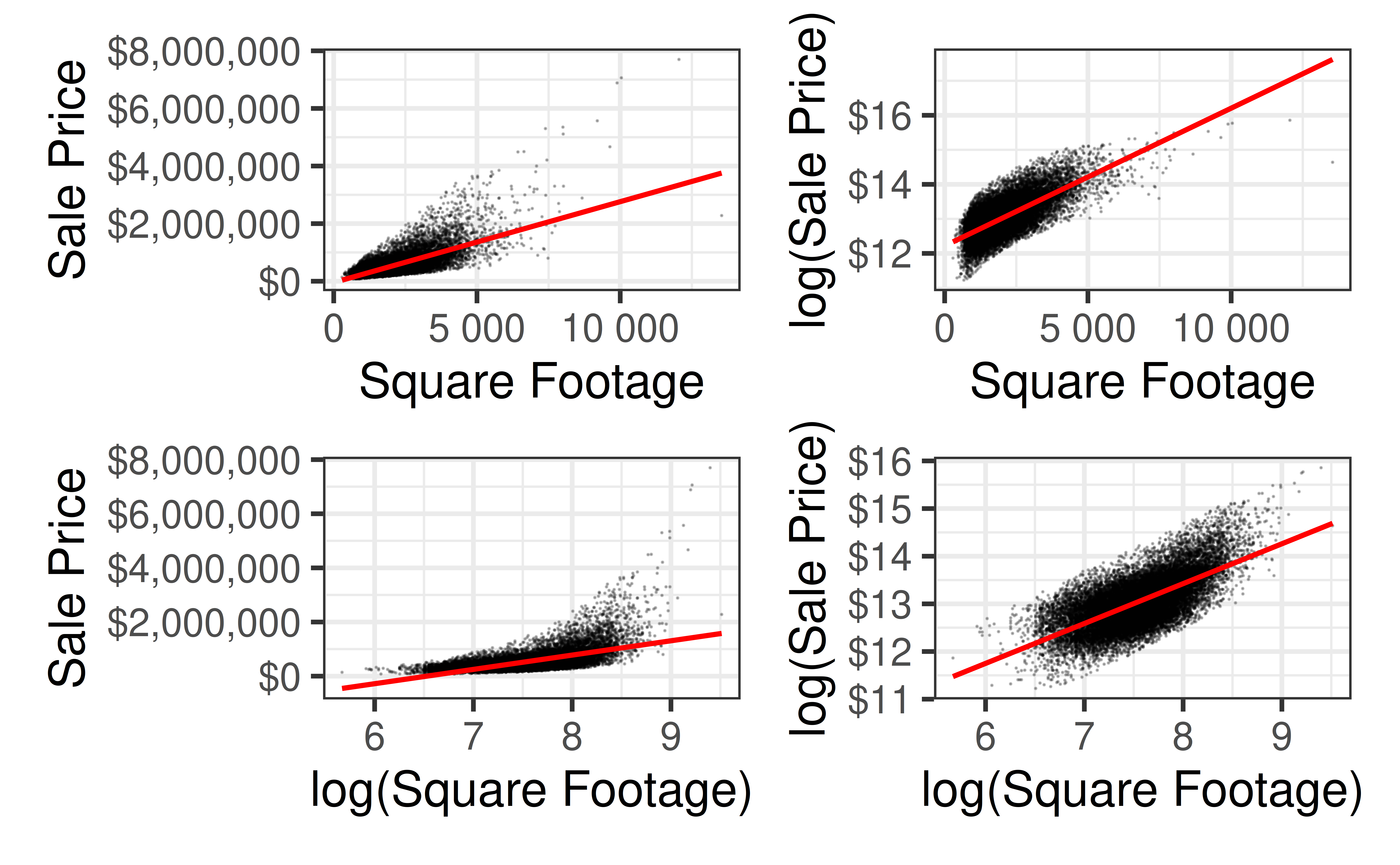
SLR: Transformations

Prof. Eric Friedlander

Application exercise

📋 AE 10/11 - Transformations + Outliers: Complete in Deepnote

Complete Exercises 0-3.

Computational set up

# load packages
library(tidyverse)   # for data wrangling and visualization
library(broom)       # for formatting model output
library(ggformula)   # for creating plots using formulas
library(scales)      # for pretty axis labels
library(knitr)       # for pretty tables
library(moderndive)  # for house_price dataset
library(fivethirtyeight)   # for fandango dataset
library(kableExtra)  # also for pretty tables
library(patchwork)   # arrange plots

# set default theme and larger font size for ggplot2
ggplot2::theme_set(ggplot2::theme_bw(base_size = 20))

Data: `house_prices`

Contains house sale prices for King County, which includes Seattle, from homes sold between May 2014 and May 2015
Obtained from Kaggle.com
Imported from the moderndive package

glimpse(house_prices)

Rows: 21,613
Columns: 21
$ id            <chr> "7129300520", "6414100192", "5631500400", "2487200875", …
$ date          <date> 2014-10-13, 2014-12-09, 2015-02-25, 2014-12-09, 2015-02…
$ price         <dbl> 221900, 538000, 180000, 604000, 510000, 1225000, 257500,…
$ bedrooms      <int> 3, 3, 2, 4, 3, 4, 3, 3, 3, 3, 3, 2, 3, 3, 5, 4, 3, 4, 2,…
$ bathrooms     <dbl> 1.00, 2.25, 1.00, 3.00, 2.00, 4.50, 2.25, 1.50, 1.00, 2.…
$ sqft_living   <int> 1180, 2570, 770, 1960, 1680, 5420, 1715, 1060, 1780, 189…
$ sqft_lot      <int> 5650, 7242, 10000, 5000, 8080, 101930, 6819, 9711, 7470,…
$ floors        <dbl> 1.0, 2.0, 1.0, 1.0, 1.0, 1.0, 2.0, 1.0, 1.0, 2.0, 1.0, 1…
$ waterfront    <lgl> FALSE, FALSE, FALSE, FALSE, FALSE, FALSE, FALSE, FALSE, …
$ view          <int> 0, 0, 0, 0, 0, 0, 0, 0, 0, 0, 0, 0, 0, 0, 0, 3, 0, 0, 0,…
$ condition     <fct> 3, 3, 3, 5, 3, 3, 3, 3, 3, 3, 3, 4, 4, 4, 3, 3, 3, 4, 4,…
$ grade         <fct> 7, 7, 6, 7, 8, 11, 7, 7, 7, 7, 8, 7, 7, 7, 7, 9, 7, 7, 7…
$ sqft_above    <int> 1180, 2170, 770, 1050, 1680, 3890, 1715, 1060, 1050, 189…
$ sqft_basement <int> 0, 400, 0, 910, 0, 1530, 0, 0, 730, 0, 1700, 300, 0, 0, …
$ yr_built      <int> 1955, 1951, 1933, 1965, 1987, 2001, 1995, 1963, 1960, 20…
$ yr_renovated  <int> 0, 1991, 0, 0, 0, 0, 0, 0, 0, 0, 0, 0, 0, 0, 0, 0, 0, 0,…
$ zipcode       <fct> 98178, 98125, 98028, 98136, 98074, 98053, 98003, 98198, …
$ lat           <dbl> 47.5112, 47.7210, 47.7379, 47.5208, 47.6168, 47.6561, 47…
$ long          <dbl> -122.257, -122.319, -122.233, -122.393, -122.045, -122.0…
$ sqft_living15 <int> 1340, 1690, 2720, 1360, 1800, 4760, 2238, 1650, 1780, 23…
$ sqft_lot15    <int> 5650, 7639, 8062, 5000, 7503, 101930, 6819, 9711, 8113, …

Variables

Outcome
- price: the sale price in dollars
Predictor
- sqft_living: the square footage of the home

Recap: Fit the model

hp_fit <- lm(price ~ sqft_living, data = house_prices)
tidy(hp_fit) |>  kable()

term	estimate	std.error	statistic	p.value
(Intercept)	-43580.7431	4402.689690	-9.898663	0
sqft_living	280.6236	1.936399	144.920356	0

Write down the model:
- Model: $\hat{\text{price}} = -43580.74 + 280.62\times\text{sqft_living}$
Interpret the slope and intercept in the context of this problem:
- Interpretation: If the square footage of the house increases by 1, the price increases by and average of $280.62 and a (theoretical) house with 0 square feet with cost -$43,580.74.

Recap: Fit the model

Code

gf_point(price ~ sqft_living, data = house_prices,
         alpha = 0.25, size = 0.01) |> 
  gf_smooth(method = "lm", color = "red") |> 
  gf_labs(x = "Square Footage", 
       y = "Sale Price")  |> 
  gf_refine(scale_y_continuous(labels = label_dollar()),
  scale_x_continuous(labels = label_number()))

Recap: Model conditions

Linearity: There is a linear relationship between the outcome and predictor variables
Constant variance: The variability of the errors is equal for all values of the predictor variable
Normality: The errors follow a normal distribution
Independence: The errors are independent from each other

How should we check these assumptions?

Recap: Residual Histogram

Code

hp_aug <- augment(hp_fit)

gf_histogram(~.resid, data = hp_aug, bins = 100) |> 
  gf_labs(x = "Residual", 
       y = "Count", 
       title = "Residual Histogram")

Recap: QQ-Plot of Residuals

Code

gf_qq(~.resid, data = hp_aug) |> 
  gf_qqline() |>
  gf_labs(x = "Theoretical quantile", 
       y = "Observed quantile", 
       title = "Normal QQ-plot of residuals")

Recap: Residuals vs. Fitted Values

Code

gf_point(.resid ~ .fitted, data = hp_aug, 
         alpha = 0.25, size = 0.01) |> 
  gf_hline(yintercept = 0, linetype = "dashed") |> 
  gf_labs(
    x = "Fitted value", y = "Residual",
    title = "Residuals vs. fitted values"
  )

Are model conditions satisfied?

Linearity: ❓
Constant variance: ❌
Normality: ❌
Independence: ❓

What to do when regression conditions are violated

Examples:

Lack of normality in residuals
Patterns in residuals
Heteroscedasticity (non-constant variance)
Outliers: influential points, large residuals

Transformations

Data Transformations

Can be used to:

Address nonlinear patterns
Stabilize variance
Remove skewness from residuals
Minimize effects of outliers

Common Transformations

For either the response $Y$ or predictor $X$:

Logarithm $Z \to \log(Z)$
- Note: “log” means “log base $e$”
Square Root $Z \to \sqrt{Z}$
Exponential $Z \to e^Z$
Power functions $Z \to Z^2, Z^3, Z^4, \ldots$
Reciprocal $Z \to 1/Z$

General Approach

Fix non-constant variance by transforming $Y$ (do this first)
- Fan Pattern: Log-Transform $Y$
Fix non-linearity by transforming $X$

Why a Log Transformation?

Some relationship are multiplicative (not linear)

Example: Area of a circle

\[ \begin{aligned} A &= \pi r^2 \text{ (not linear)}\\ \log(A) &= \log(\pi r^2) = \log(\pi) + 2\log(r)\\ \log(A) &= \beta_0 + \beta_1\times \log(r)\\ \implies & \log(A) \text{ is a linear function of } \log(r) \end{aligned} \]

Look for:

Increasing variability in scatterplot
Strongly right-skewed residual distributions
Complete Exercise 4

Fixing non-linearity

Many departures from linearity can be solved with power transformations (e.g. $X^{power}$)
- For technical reasons, $power = 0$ corresponds to $\log$
Concave down pattern $\Rightarrow$ transform down (i.e. $power < 1$)
- $\log$ is typically a good first choice
Concave up pattern $\Rightarrow$ transform up (i.e. $power > 1$)
Complete Exercises 5-7.

Back to `house_sales`

Code

p1 <- gf_point(price ~ sqft_living, data = house_prices,
         alpha = 0.25, size = 0.01) |> 
  gf_smooth(method = "lm", color = "red") |> 
  gf_labs(x = "Square Footage", 
       y = "Sale Price")  |> 
  gf_refine(scale_y_continuous(labels = label_dollar()),
  scale_x_continuous(labels = label_number()))

p2 <- gf_point(log(price) ~ sqft_living, data = house_prices,
         alpha = 0.25, size = 0.01) |> 
  gf_smooth(method = "lm", color = "red") |> 
  gf_labs(x = "Square Footage", 
       y = "log(Sale Price)")  |> 
  gf_refine(scale_y_continuous(labels = label_dollar()),
  scale_x_continuous(labels = label_number()))

p3 <- gf_point(price ~ log(sqft_living), data = house_prices,
         alpha = 0.25, size = 0.01) |> 
  gf_smooth(method = "lm", color = "red") |> 
  gf_labs(x = "log(Square Footage)", 
       y = "Sale Price")  |> 
  gf_refine(scale_y_continuous(labels = label_dollar()),
  scale_x_continuous(labels = label_number()))

p4 <- gf_point(log(price) ~ log(sqft_living), data = house_prices,
         alpha = 0.25, size = 0.01) |> 
  gf_smooth(method = "lm", color = "red") |> 
  gf_labs(x = "log(Square Footage)", 
       y = "log(Sale Price)")  |> 
  gf_refine(scale_y_continuous(labels = label_dollar()),
  scale_x_continuous(labels = label_number()))

(p1 + p2)/ (p3 + p4)

Fitting Transformed Models

logprice_model <- lm(log(price) ~ sqft_living, data = house_prices)
tidy(logprice_model) |> kable()

term	estimate	std.error	statistic	p.value
(Intercept)	12.2184641	0.0063741	1916.8830	0
sqft_living	0.0003987	0.0000028	142.2326	0

\[ \begin{aligned} \log(Y) &= 12.22 + 3.99\times 10^{-4}\times X\\ Y &= e^{12.22 + 3.99\times 10^{-4}\times X}\\ &= 202805\times e^{3.99\times 10^{-4}\times X} \end{aligned} \]

loglog_model <- lm(log(price) ~ log(sqft_living), data = house_prices)
tidy(loglog_model) |> kable()

term	estimate	std.error	statistic	p.value
(Intercept)	6.729916	0.0470620	143.0011	0
log(sqft_living)	0.836771	0.0062233	134.4587	0

\[ \begin{aligned} \log(Y) &=6.73 + 0.837\times \log(X)\\ \log(Y) &= \log(e^{6.73}) + \log(X^{0.837})\\ Y &= 873.15\times X^{0.837} \end{aligned} \]

Residuals Histograms

Code

lp_aug <- augment(logprice_model)
ll_aug <- augment(loglog_model)

p1 <- gf_histogram(~.resid, data = lp_aug, bins = 100) |> 
  gf_labs(x = "Residual", 
       y = "Count", 
       title = "Log Price Residuals")

p2 <- gf_histogram(~.resid, data = ll_aug, bins = 100) |> 
  gf_labs(x = "Residual", 
       y = "Count", 
       title = "Log-Log Residuals")

(p1 + p2)

QQ-Plots of Residuals

Code

p1 <- gf_qq(~.resid, data = lp_aug) |> 
  gf_qqline() |>
  gf_labs(x = "Theoretical quantile", 
       y = "Observed quantile", 
       title = "Log Price QQ")

p2 <- gf_qq(~.resid, data = ll_aug) |> 
  gf_qqline() |>
  gf_labs(x = "Theoretical quantile", 
       y = "Observed quantile", 
       title = "Log-Log QQ")

p1 + p2

Residuals vs. Fitted Values

Code

p1 <- gf_point(.resid ~ .fitted, data = lp_aug, 
         alpha = 0.25, size = 0.01) |> 
  gf_hline(yintercept = 0, linetype = "dashed") |> 
  gf_labs(
    x = "Fitted value", y = "Residual",
    title = "Log Price Model"
  )

p2 <- gf_point(.resid ~ .fitted, data = ll_aug, 
         alpha = 0.25, size = 0.01) |> 
  gf_hline(yintercept = 0, linetype = "dashed") |> 
  gf_labs(
    x = "Fitted value", y = "Residual",
    title = "Log-Log Model"
  )

p1 + p2

A note on evaluation

If you are computing your evaluation metrics (e.g. $R^2$ or RMSE), you should transform your predictions BACK to their original scale, especially if you’re trying to choose the best model

Why do we need to undo the transformation for evaluation metrics by not residuals plots?
Why don’t we need to worry about the predictors?

Recap

Transformations
- Transform $Y$ to fix non-constant variance (and non-normality)
- Transform $X$ to fix non-linearity
- Power transformations are powerful (concave up/drown $\Rightarrow$ power up/down)
- logs allow us to model a lot of non-linear relationships with a linear model

SLR: Transformations

Application exercise

Computational set up

Data: house_prices

Variables

Recap: Fit the model

Recap: Fit the model

Recap: Model conditions

Recap: Residual Histogram

Recap: QQ-Plot of Residuals

Recap: Residuals vs. Fitted Values

Are model conditions satisfied?

What to do when regression conditions are violated

Transformations

Data Transformations

Common Transformations

General Approach

Why a Log Transformation?

Fixing non-linearity

Back to house_sales

Fitting Transformed Models

Residuals Histograms

QQ-Plots of Residuals

Residuals vs. Fitted Values

A note on evaluation

Recap

Data: `house_prices`

Back to `house_sales`