Goal: Use the average household income to understand variation in access to organic foods.
Computational setup
# load packageslibrary(tidyverse) # for data wrangling library(ggformula) # for visualizing datalibrary(broom) # for nicely displaying modelslibrary(mosaic) # for shufflinglibrary(scales) # for pretty axis labelslibrary(knitr) # for neatly formatted tableslibrary(kableExtra) # also for neatly formatted tables# set default theme and larger font size for ggplot2ggplot2::theme_set(ggplot2::theme_bw(base_size =16))
Exploratory data analysis
Code
heb <-read_csv(here::here("data/HEBIncome.csv")) |>mutate(Avg_Income_K = Avg_Household_Income/1000)gf_point(Number_Organic ~ Avg_Income_K, data = heb, alpha =0.7) |>gf_labs(x ="Average Household Income (in thousands)",y ="Number of Organic Vegetables", ) |>gf_refine(scale_x_continuous(labels =label_dollar()))
Modeling
heb_fit <-lm(Number_Organic ~ Avg_Income_K, data = heb)tidy(heb_fit)
Intercept: HEBs in Zip Codes with an average household income of $0 are expected to have -14.72 organic vegetable options, on average.
Is this interpretation useful?
Slope: For each additional $1,000 in average household income, we expect the number of organic options available at nearby HEBs to increase by 0.96, on average.
From sample to population
For each additional $1,000 in average household income, we expect the number of organic options available at nearby HEBs to increase by 0.96, on average.
Estimate is valid for the single sample of 37 HEBs
What if we’re not interested quantifying the relationship between the household income and access to organic vegetables in this single sample?
What if we want to say something about the relationship between these variables for all supermarkets in America?
Statistical inference
Statistical inference refers to ideas, methods, and tools for generalizing the single observed sample to make statements (inferences) about the population it comes from
For our inferences to be valid, the sample should be random and representative of the population we’re interested in
Sampling is natural
When you taste a spoonful of soup and decide the spoonful you tasted isn’t salty enough, that’s exploratory analysis
If you generalize and conclude that your entire soup needs salt, that’s an inference
For your inference to be valid, the spoonful you tasted (the sample) needs to be representative of the entire pot (the population)
Inference for simple linear regression
Conduct a hypothesis test for the slope, \(\beta_1\)
Why not \(\beta_0\)?
We can but it isn’t super interesting typically
Calculate a confidence interval for the slope, \(\beta_1\)
What is a confidence interval?
What is a hypothesis test?
Research question and hypotheses
“Do the data provide sufficient evidence that \(\beta_1\) (the true slope for the population) is different from 0?”
Null hypothesis: there is no linear relationship between Number_Organic and Avg_Income_K
\[
H_0: \beta_1 = 0
\]
Alternative hypothesis: there is a linear relationship between Number_Organic and Avg_Income_K
\[
H_A: \beta_1 \ne 0
\]
Hypothesis testing as a court trial
Null hypothesis, \(H_0\): Defendant is innocent
Alternative hypothesis, \(H_A\): Defendant is guilty
Present the evidence: Collect data
Judge the evidence: “Could these data plausibly have happened by chance if the null hypothesis were true?”
Yes: Fail to reject \(H_0\)
No: Reject \(H_0\)
Not guilty \(\neq\) innocent \(\implies\) why we say “fail to reject the null” rather than “accept the null”
Hypothesis testing framework
Start with a null hypothesis, \(H_0\) that represents the status quo
Set an alternative hypothesis, \(H_A\) that represents the research question, i.e. claim we’re testing
Under the assumption that the null hypothesis is true, calculate a p-value (probability of getting outcome or outcome even more favorable to the alternative)
if the test results suggest that the data do not provide convincing evidence for the alternative hypothesis, stick with the null hypothesis
if they do, then reject the null hypothesis in favor of the alternative
Complete Exercise 3.
Quantify the variability of the slope
for testing
Two approaches:
Via simulation
Via mathematical models
Use Randomization to quantify the variability of the slope for the purpose of testing, under the assumption that the null hypothesis is true:
Simulate new samples from the original sample via permutation
Fit models to each of the samples and estimate the slope
Use features of the distribution of the permuted slopes to conduct a hypothesis test
Permutation, described
Use permuting to simulate data under the assumption the null hypothesis is true and measure the natural variability in the data due to sampling, not due to variables being correlated
Permute/shuffle response variable to eliminate any existing relationship with explanatory variable
Each Number_Organic value is randomly assigned to the Avg_Household_K, i.e. Number_Organic and Avg_Household_K are no longer matched for a given store
Each of the observed values for Number_Organic (and for Avg_Income_K) exist in both the observed data plot as well as the permuted Number_Organic plot
Permuting removes the relationship between Number_Organic and Avg_Income_K
Permutation, repeated
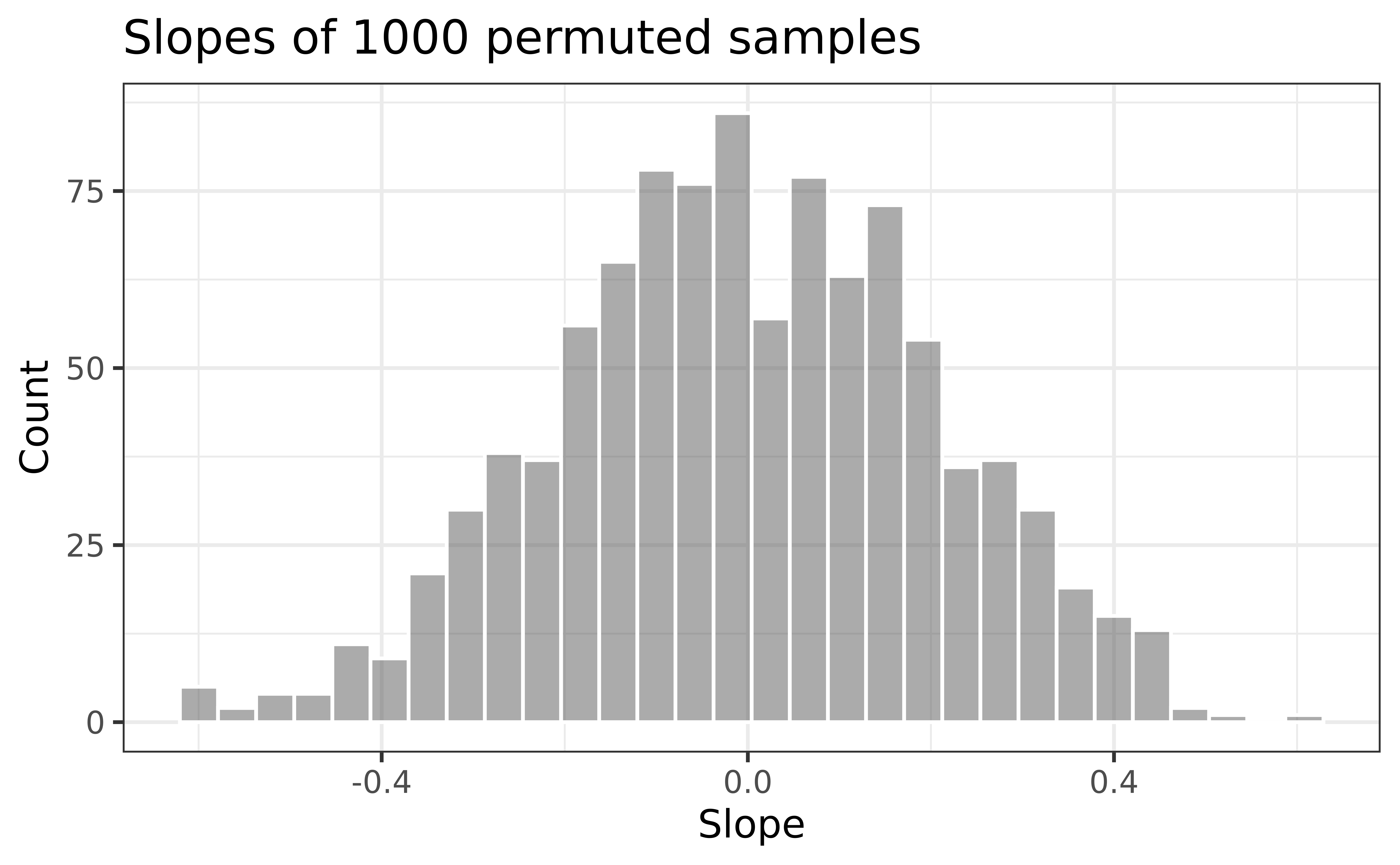
Repeated permutations allow for quantifying the variability in the slope under the condition that there is no linear relationship (i.e., that the null hypothesis is true)
Concluding the hypothesis test
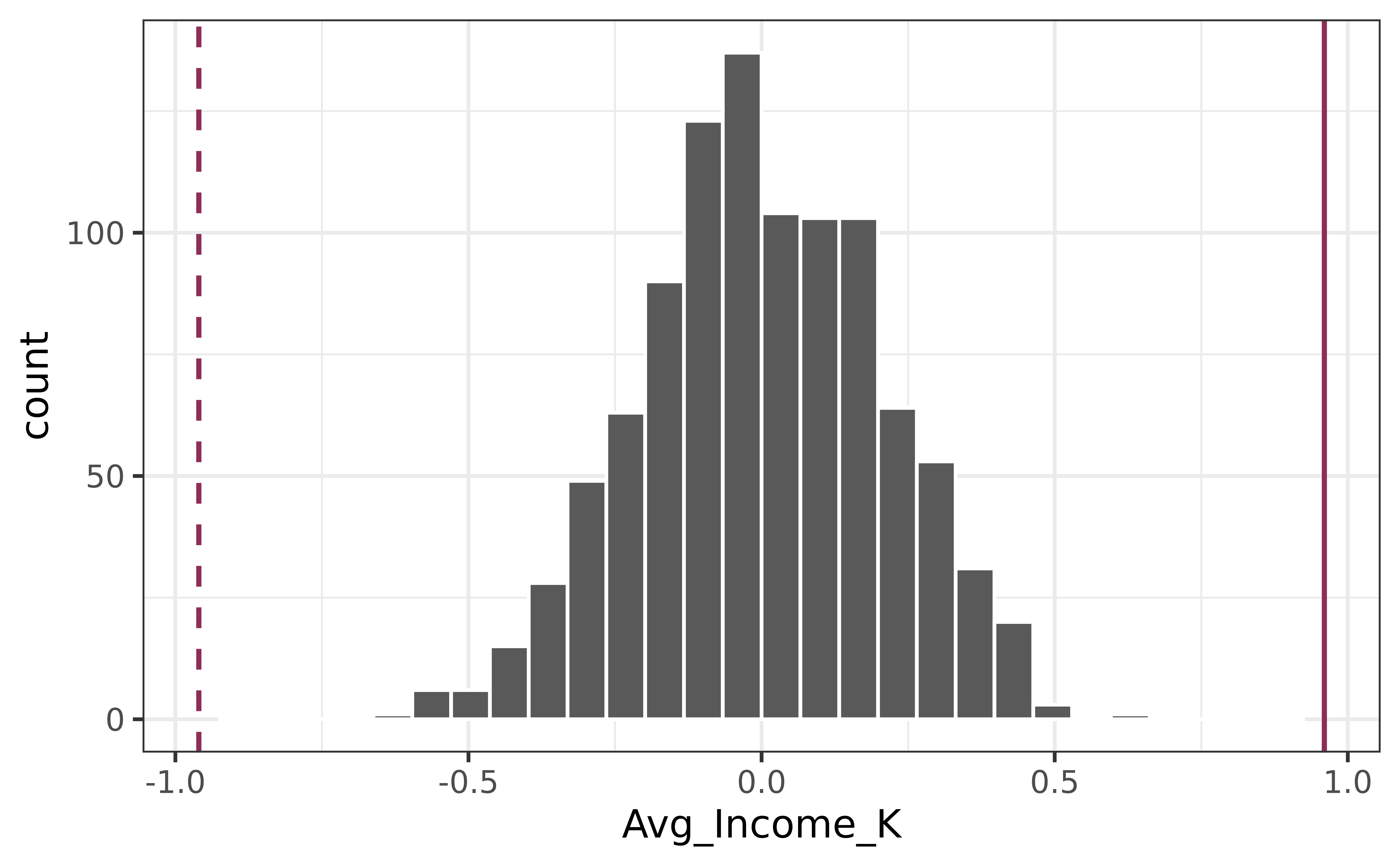
Is the observed slope of \(\hat{\beta_1} = 0.96\) (or an even more extreme slope) a likely outcome under the null hypothesis that \(\beta = 0\)? What does this mean for our original question: “Do the data provide sufficient evidence that \(\beta_1\) (the true slope for the population) is different from 0?”
Regular Model
set.seed(1218)lm(Number_Organic ~ Avg_Income_K, data = heb)
set.seed(1218)null_dist <-do(1000) *lm(shuffle(Number_Organic) ~ Avg_Income_K, data = heb)
Visualize the null distribution
null_dist |>gf_histogram(~Avg_Income_K, color ="white") |>gf_labs(x ="Slope",y ="Count",title ="Slopes of 1000 permuted samples" )
Complete Exercises 5-7.
Reason around the p-value
In a world where there is no relationship between the number of organic food options and the nearby average household income (\(\beta_1 = 0\)), what is the probability that we observe a sample of 37 stores where the slope of the model predicting the number of organic options from average household income is 0.96 or even more extreme?
Compute the p-value
# fit model to get observed slopelm(Number_Organic ~ Avg_Income_K, data = heb) |>tidy()
# mean treats trues and falses like 1's and zeros (this is our p-value)mean(abs(null_dist$Avg_Income_K) >=abs(0.9591))
[1] 0
Complete Exercises 8 and 9.
Recap
Population: Complete set of observations of whatever we are studying, e.g., people, tweets, photographs, etc. (population size = \(N\))
Sample: Subset of the population, ideally random and representative (sample size = \(n\))
Sample statistic \(\ne\) population parameter, but if the sample is good, it can be a good estimate
Permutation and refitting (using mosaic): Use repeated shuffling and model fitting to understand how sample statistics vary due to random chance, helping us extract meaning and information from data generated by random processes.
Recap Continued
Testing: Conduct a hypothesis test
Assume research question isn’t true (Null hypothesis)
Ask what distribution of test statistic is if null is true
Ask if your data would be unusual if under this null distribution
P-value: Probability your data (or even stronger evidence) was obtained from null distribution