# load packages
library(tidyverse)       # for data wrangling
library(ggformula)       # for plotting
library(broom)           # for formatting model output
library(knitr)           # for formatting tables

# set default theme and larger font size for ggplot2
ggplot2::theme_set(ggplot2::theme_bw(base_size = 16))

# set default figure parameters for knitr
knitr::opts_chunk$set(
  fig.width = 8,
  fig.asp = 0.618,
  fig.retina = 3,
  dpi = 300,
  out.width = "80%"
)Simple Linear Regression
Prof. Eric Friedlander
Introduction to Simple Linear Regression
Topics
Interpret the slope and intercept of the regression line.
Use R to fit and summarize regression models.
Computation set up
Recap
DC Bikeshare
Our data set contains daily rentals from the Capital Bikeshare in Washington, DC in 2011 and 2012. It was obtained from the dcbikeshare data set in the dsbox R package.
We will focus on the following variables in the analysis:
count: total bike rentalstemp_orig: Temperature in degrees Celsiusseason: 1 - winter, 2 - spring, 3 - summer, 4 - fall
Click here for the full list of variables and definitions.
Data prep
- Converted
seasonfrom 1, 2, 3, 5 into “winter”, “spring”, “summer”, “fall” and convered it into afactor - Created a new dataset called
winterthat contains only thewintermonths
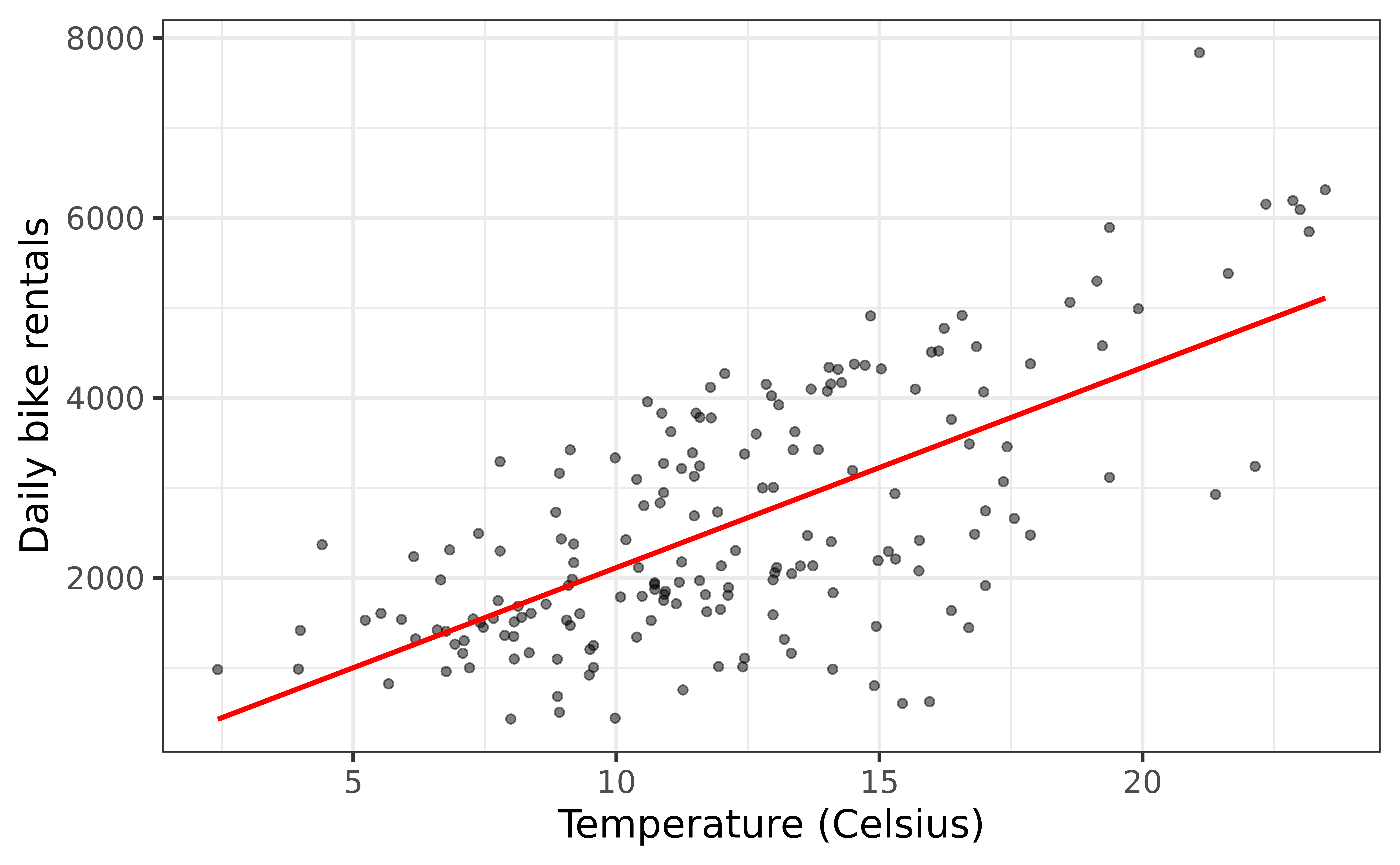
Rentals vs Temperature
Goal: Fit a line to describe the relationship between the temperature and the number of rentals in winter.
Residuals
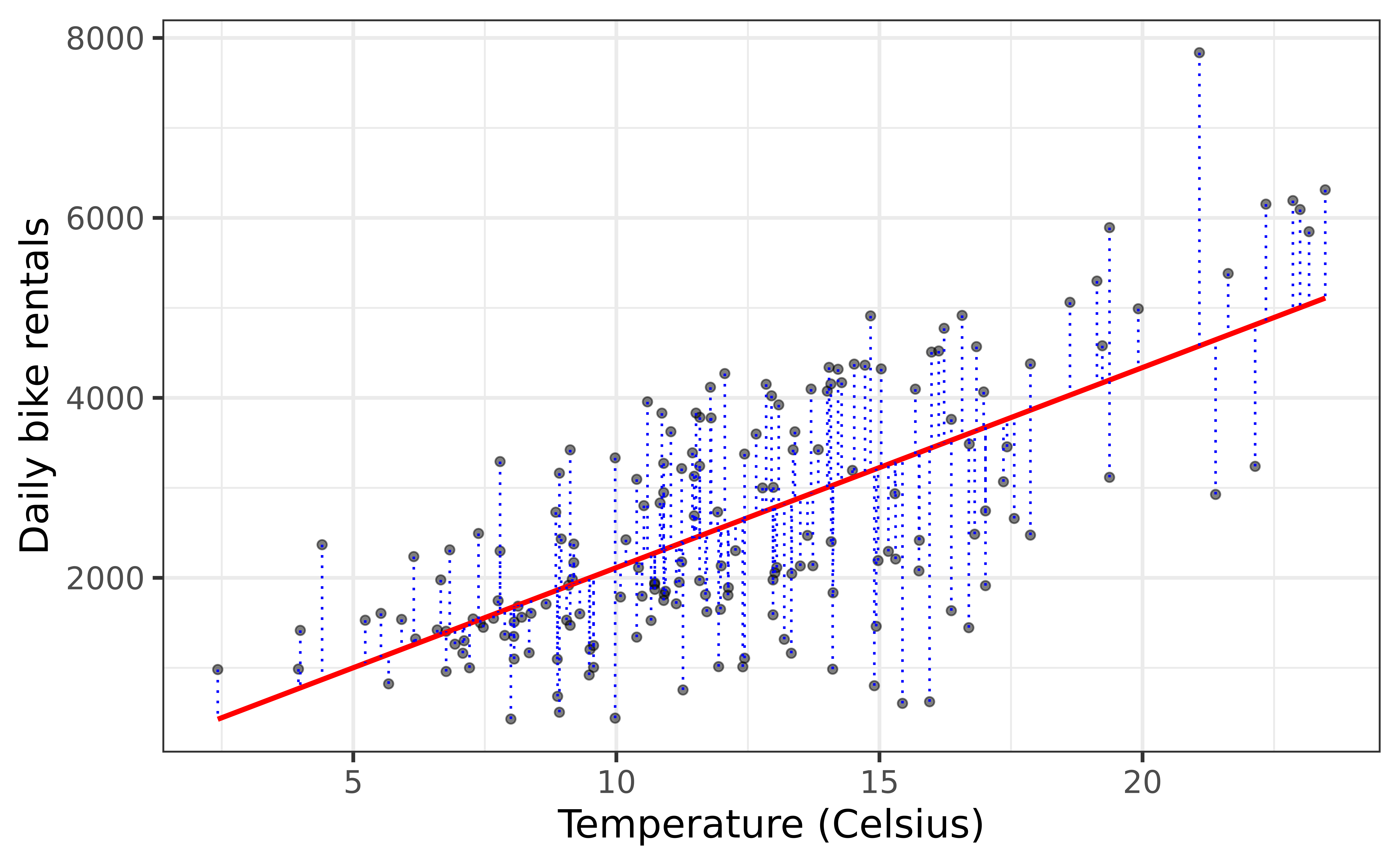
\[\text{residual} = \text{observed} - \text{predicted} = y_i - \hat{y}_i\]
Last Time
- Sample: data that you have
- Population: group you trying to generalize to
- Representative sample: when your sample looks like small version of your population, if not, we say it’s a biased sample
- Simple linear regression (SLR): assume relationship betweenquantitative predictor (\(X\)) and response (\(Y\)) is a line:
- Statistical model: \(Y = \mathbf{\beta_0 + \beta_1 X} + \epsilon\)
- The regression equation: \(\hat{Y} = \hat{\beta}_0 + \hat{\beta}_1 X\)
- \(\hat{\beta}_1\) (slope): estimated change in \(Y\) for each unit increase in \(X\)
- \(\hat{\beta}_0\) (intercept): estimated value of \(Y\) when \(X = 0\)
- Residuals: difference between observed and predicted values (\(e_i = y_i - \hat{y}_i\))
- Least squares method chooses coefficients to minimize the sum of squared residuals
- SLR can be used for prediction and inference
Slope and intercept
Properties of least squares regression
Passes through center of mass point, the coordinates corresponding to average \(X\) and average \(Y\): \(\hat{\beta}_0 = \bar{Y} - \hat{\beta}_1\bar{X}\)
Slope has same sign as the correlation coefficient: \(\hat{\beta}_1 = r \frac{s_Y}{s_X}\)
- \(r\): correlation coefficient
- \(s_Y, s_X\): sample standard deviations of \(X\) and \(Y\)
Sum of the residuals is zero: \(\sum_{i = 1}^n e_i \approx 0\)
- Intuition: Residuals are “balanced”
The residuals and \(X\) values are uncorrelated
Estimating the slope
\[\large{\hat{\beta}_1 = r \frac{s_Y}{s_X}}\]
\[\begin{aligned}
s_X &= 4.2121 \\
s_Y &= 1399.942 \\
r &= 0.6692
\end{aligned}\]
\[\begin{aligned}
\hat{\beta}_1 &= 0.6692 \times \frac{1399.942}{4.2121} \\
&= 222.417\end{aligned}\]
Click here for details on deriving the equations for slope and intercept which is easy if you know multivariate calculus.
Estimating the intercept
\[\large{\hat{\beta}_0 = \bar{Y} - \hat{\beta}_1\bar{X}}\]
\[\begin{aligned}
&\bar{x} = 12.2076 \\
&\bar{y} = 2604.133 \\
&\hat{\beta}_1 = 222.4167
\end{aligned}\]
\[\begin{aligned}\hat{\beta}_0 &= 2604.133 - 222.4167 \times 12.2076 \\
&= -111.0411
\end{aligned}\]
Click here for details on deriving the equations for slope and intercept.
Interpretation
- Slope: For each additional unit of \(X\) we expect \(Y\) to increase by \(\hat{\beta}_1\), on average.
- Intercept: If \(X\) were 0, we predict \(Y\) to be \(\hat{\beta}_0\)
Does it make sense to interpret the intercept?
✅ The intercept is meaningful in the context of the data if
the predictor can feasibly take values equal to or near zero, or
there are values near zero in the observed data.
🛑 Otherwise, the intercept may not be meaningful!
- Note meaningful doesn’t mean wrong
Estimating the regression line in R
- Let’s complete Exercises 7-11
Fit model & estimate parameters
Look at the regression output
Call:
lm(formula = count ~ temp_orig, data = winter)

Coefficients:
(Intercept)    temp_orig
-111.0 222.4 \[\widehat{\text{count}} = -111.0 + 222.4 \times \text{temp_orig}\]
Note: The intercept is off by a tiny bit from the hand-calculated intercept, this is just due to rounding in the hand calculation.
The regression output
We’ll focus on the first column for now…
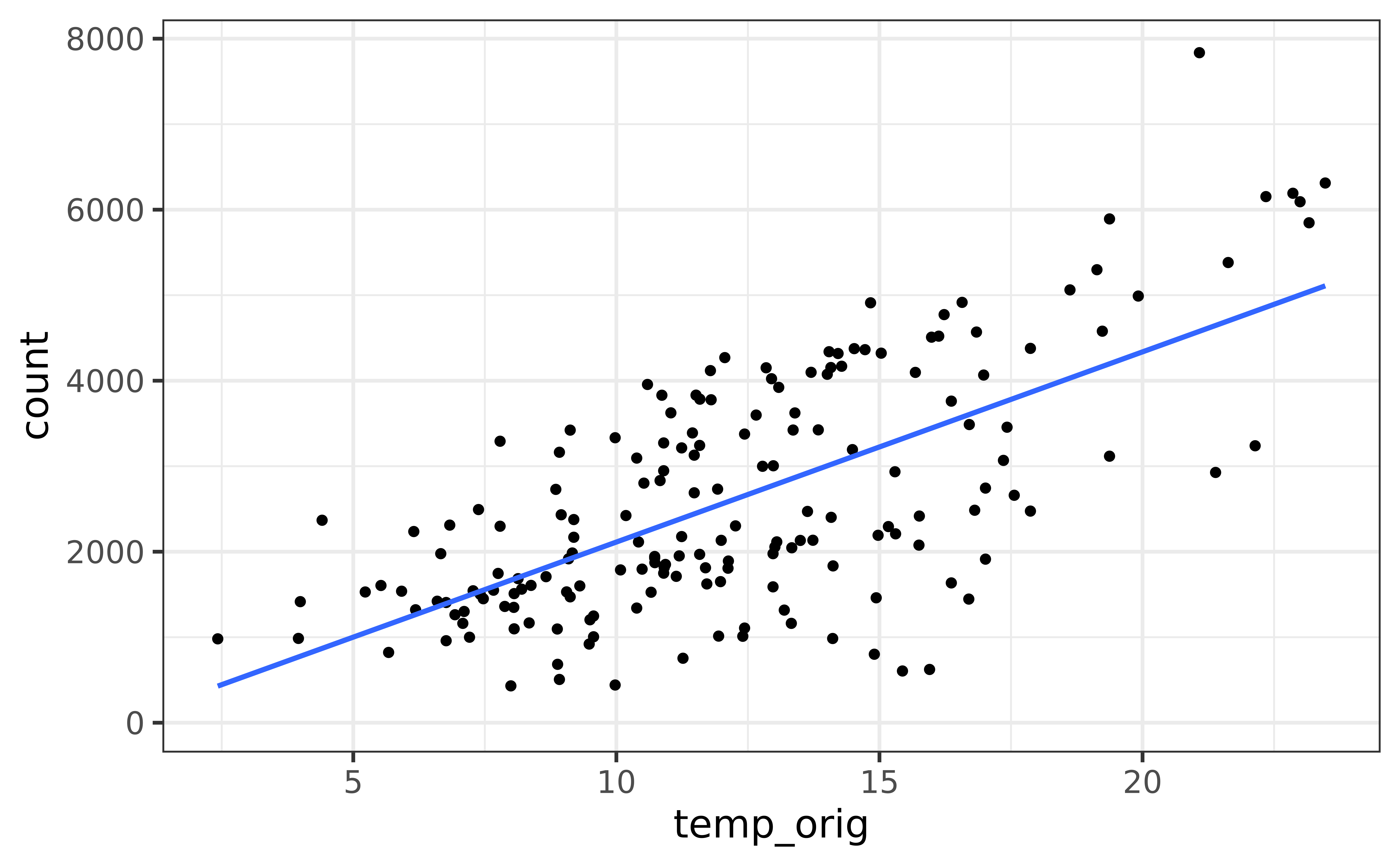
Visualize Model
Prediction
Our Model
\[\begin{aligned} \widehat{Y} &= -111.0 + 222.4 \times X\\ \widehat{\text{count}} &= -111.0 + 222.4 \times \text{temp_orig} \end{aligned}\]Making a prediction
Suppose that it’s 15 degrees Celsius outside. According to this model, how many bike rentals should we expect if it’s winter?
\[\begin{aligned} \widehat{\text{count}} &= -111.0 + 222.4 \times \text{temp_orig} \\ &= -111.0 + 222.4 \times 15 \\ &= 3225 \end{aligned}\]Prediction in R
Exercise 12
In your Deepnote project answer the following question (you’ll need to create a new markdown block):
Using only addition, subtraction, multiplication, and division. Compute the number of rentals our model would predict if it were 10 degrees Celcius outside.
Exercise 13
Verify your answer using the
predictfunction.
Recap
Used simple linear regression to describe the relationship between a quantitative predictor and quantitative response variable.
Used the least squares method to estimate the slope and intercept.
Interpreted the slope and intercept.
- Slope: For every one unit increase in \(x\), we expect y to change by \(\hat{\beta}_1\) units, on average.
- Intercept: If \(x\) is 0, then we expect \(y\) to be \(\hat{\beta}_0\) units
Predicted the response given a value of the predictor variable.
Used
lmand thebroompackage to fit and summarize regression models in R.