# load packages
library(tidyverse)       # for data wrangling
library(ggformula)       # for plotting
library(broom)           # for formatting model output
library(knitr)           # for formatting tables

# set default theme and larger font size for ggplot2
ggplot2::theme_set(ggplot2::theme_bw(base_size = 16))

# set default figure parameters for knitr
knitr::opts_chunk$set(
  fig.width = 8,
  fig.asp = 0.618,
  fig.retina = 3,
  dpi = 300,
  out.width = "80%"
)Simple Linear Regression
Application exercise
Complete Exercises 0 and 1.
Introduction to Simple Linear Regression
Topics
Use simple linear regression to describe the relationship between a quantitative predictor and quantitative response variable.
Estimate the slope and intercept of the regression line using the least squares method.
Computation set up
Data
DC Bikeshare
Our data set contains daily rentals from the Capital Bikeshare in Washington, DC in 2011 and 2012. It was obtained from the dcbikeshare data set in the dsbox R package.
We will focus on the following variables in the analysis:
count: total bike rentalstemp_orig: Temperature in degrees Celsiusseason: 1 - winter, 2 - spring, 3 - summer, 4 - fall
Click here for the full list of variables and definitions.
Let’s complete Exercises 2-6 together
Data prep
- Exercise 2: Recode
seasonas a factor with names instead of numbers (livecode) - Remember:
- Think of
|>as “and then” mutatecreates new columns and changes (mutates) existing columns- R calls categorical data “factors”
- Think of
bikeshare <- read_csv("../data/dcbikeshare.csv") |>
  mutate(season = case_when(
    season == 1 ~ "winter",
    season == 2 ~ "spring",
    season == 3 ~ "summer",
    season == 4 ~ "fall"
  ),
  season = factor(season))
Rows: 731 Columns: 17
── Column specification ────────────────────────────────────────────────────────
Delimiter: ","
dbl (16): instant, season, yr, mnth, holiday, weekday, workingday, weathers...
date (1): dteday
ℹ Use `spec()` to retrieve the full column specification for this data.
ℹ Specify the column types or set `show_col_types = FALSE` to quiet this message.Exploratory data analysis (Exercise 3)
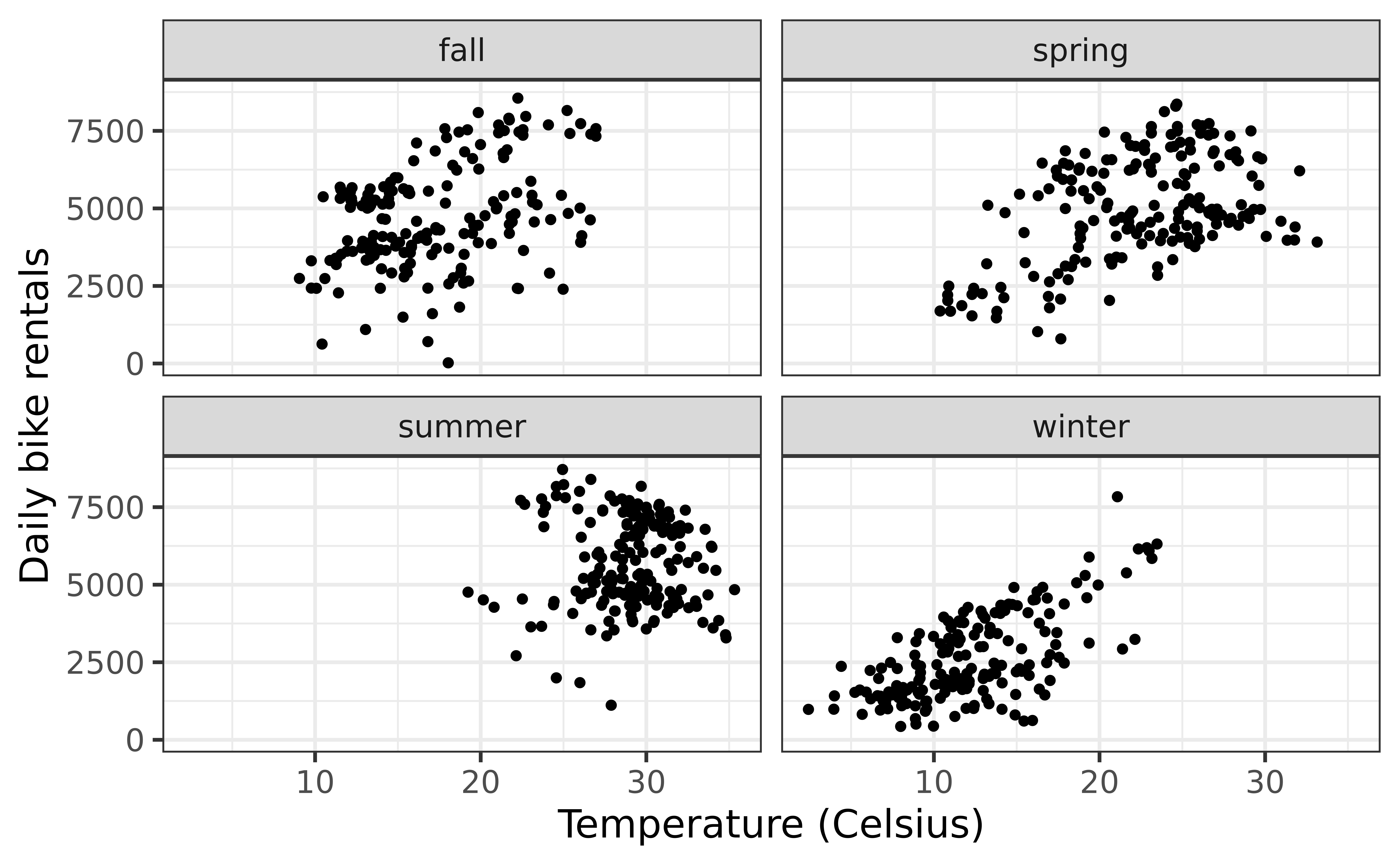
More data prep
- (Exercise 5) Filter your data for the season with the strongest relationship and give the resulting data set a new name
Rentals vs Temperature
Goal: Fit a line to describe the relationship between the temperature and the number of rentals in winter.
`geom_smooth()` using formula = 'y ~ x'
Why fit a line?
We fit a line to accomplish one or both of the following:
Prediction
How many rentals are expected when it’s 10 degrees out?
Inference
Is temperature a useful predictor of the number of rentals? By how much is the number of rentals expected to change for each degree Celsius?
Population vs. Sample
Population: The set of items or events that you’re interested in and hoping (able) to generalize the results of your analysis to.
Sample: The set of items that you have data for.
Representative Sample: A sample that looks like a small version of your population.
Goal: Build a model from your sample which generalizes to your population.
Terminology
Response, Y: variable describing the outcome of interest
Predictor, X: variable we use to help understand the variability in the response
`geom_smooth()` using formula = 'y ~ x'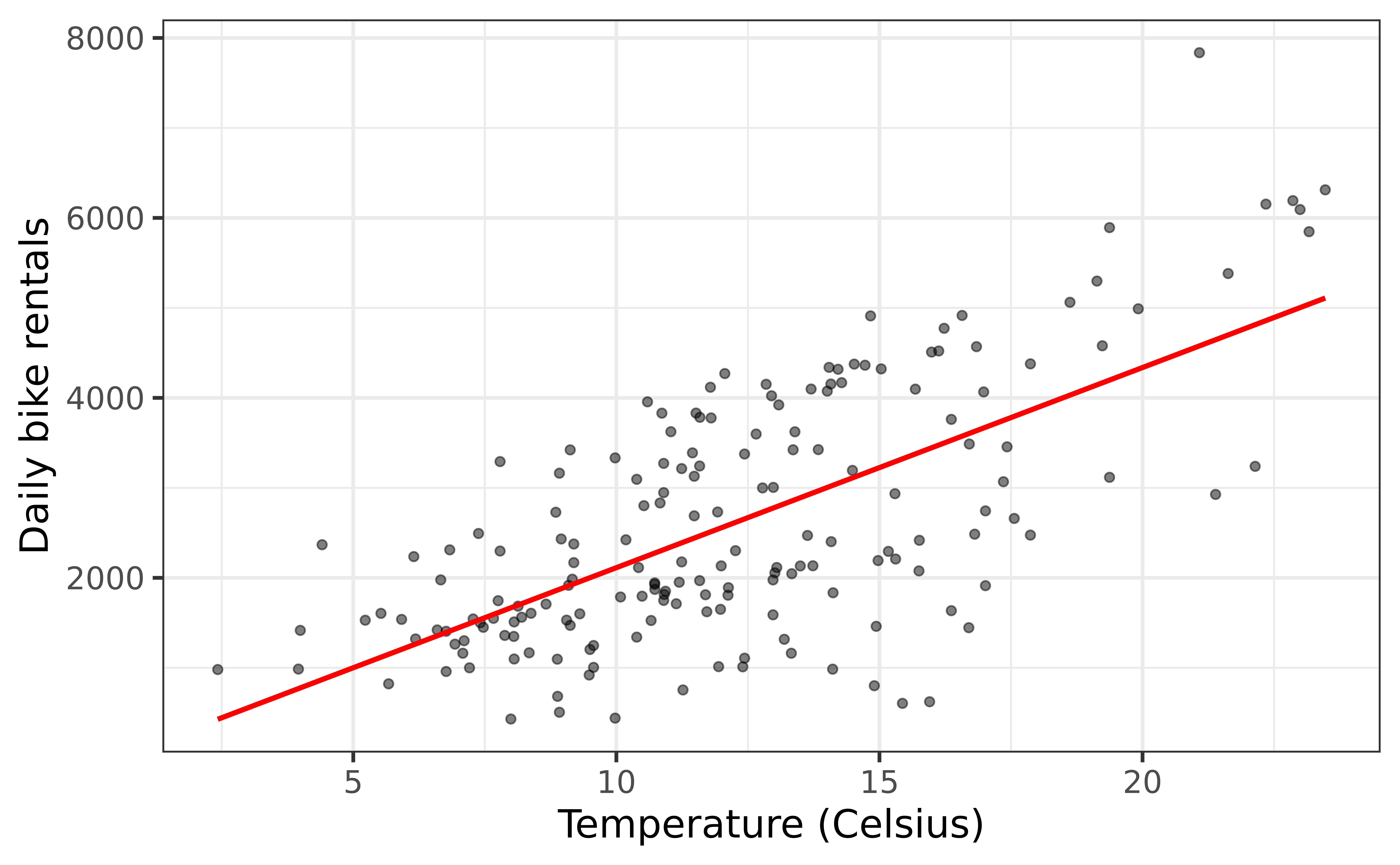
Regression model
Regression model: a function that describes the relationship between a quantitative response, \(Y\), and the predictor, \(X\) (or many predictors).
\[\begin{aligned} Y &= \color{black}{\textbf{Model}} + \text{Error} \\[8pt] &= \color{black}{\mathbf{f(X)}} + \epsilon \\[8pt] &= \color{black}{\boldsymbol{\mu_{Y|X}}} + \epsilon \end{aligned}\]Regression model
`geom_smooth()` using formula = 'y ~ x'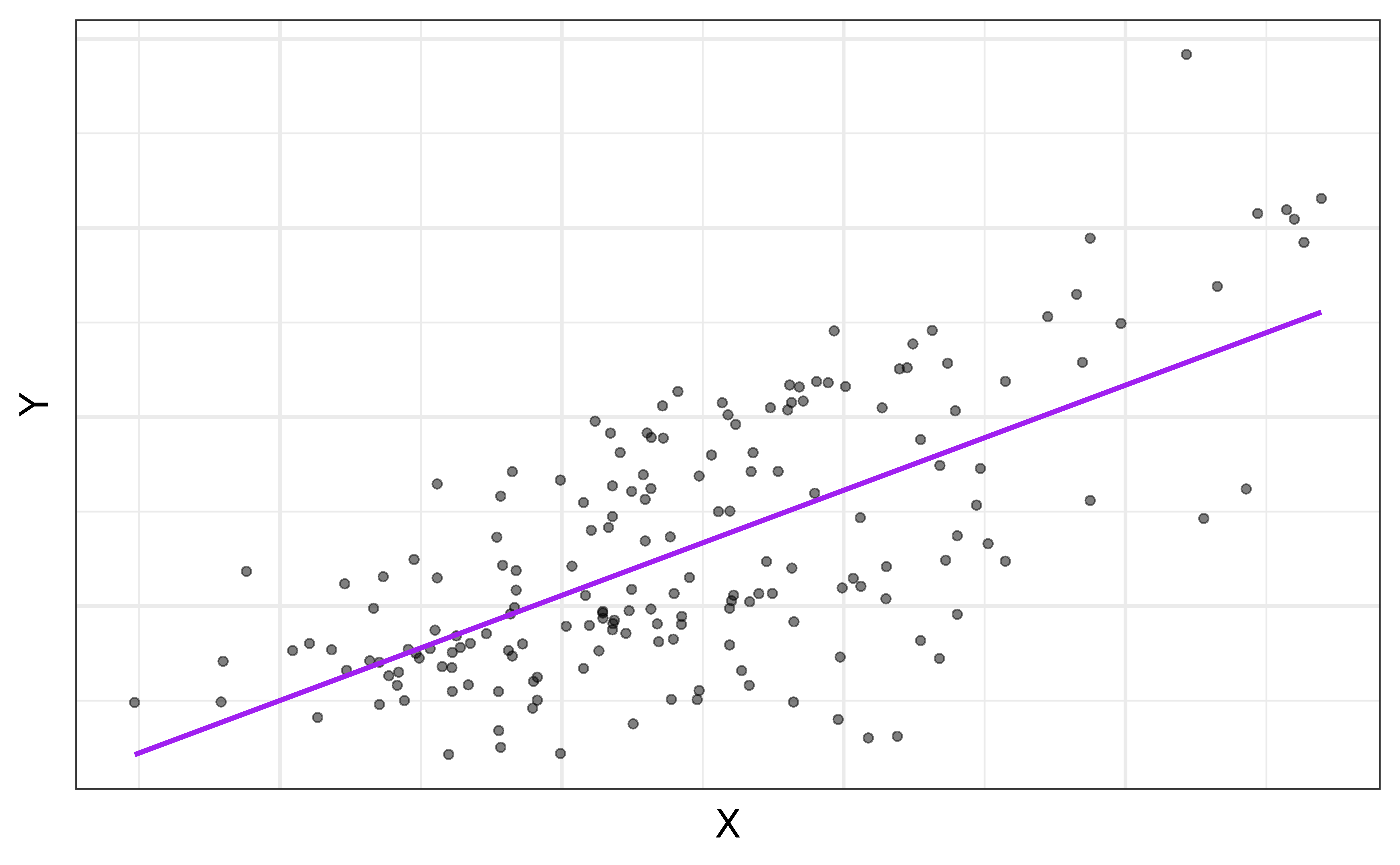
\(\mu_{Y|X}\) is the mean value of \(Y\) given a particular value of \(X\).
Regression model
\[ \begin{aligned} Y &= \color{purple}{\textbf{Model}} + \color{blue}{\textbf{Error}} \\[5pt] &= \color{purple}{\mathbf{f(X)}} + \color{blue}{\boldsymbol{\epsilon}} \\[5pt] &= \color{purple}{\boldsymbol{\mu_{Y|X}}} + \color{blue}{\boldsymbol{\epsilon}} \\[5pt] \end{aligned} \]
`geom_smooth()` using formula = 'y ~ x'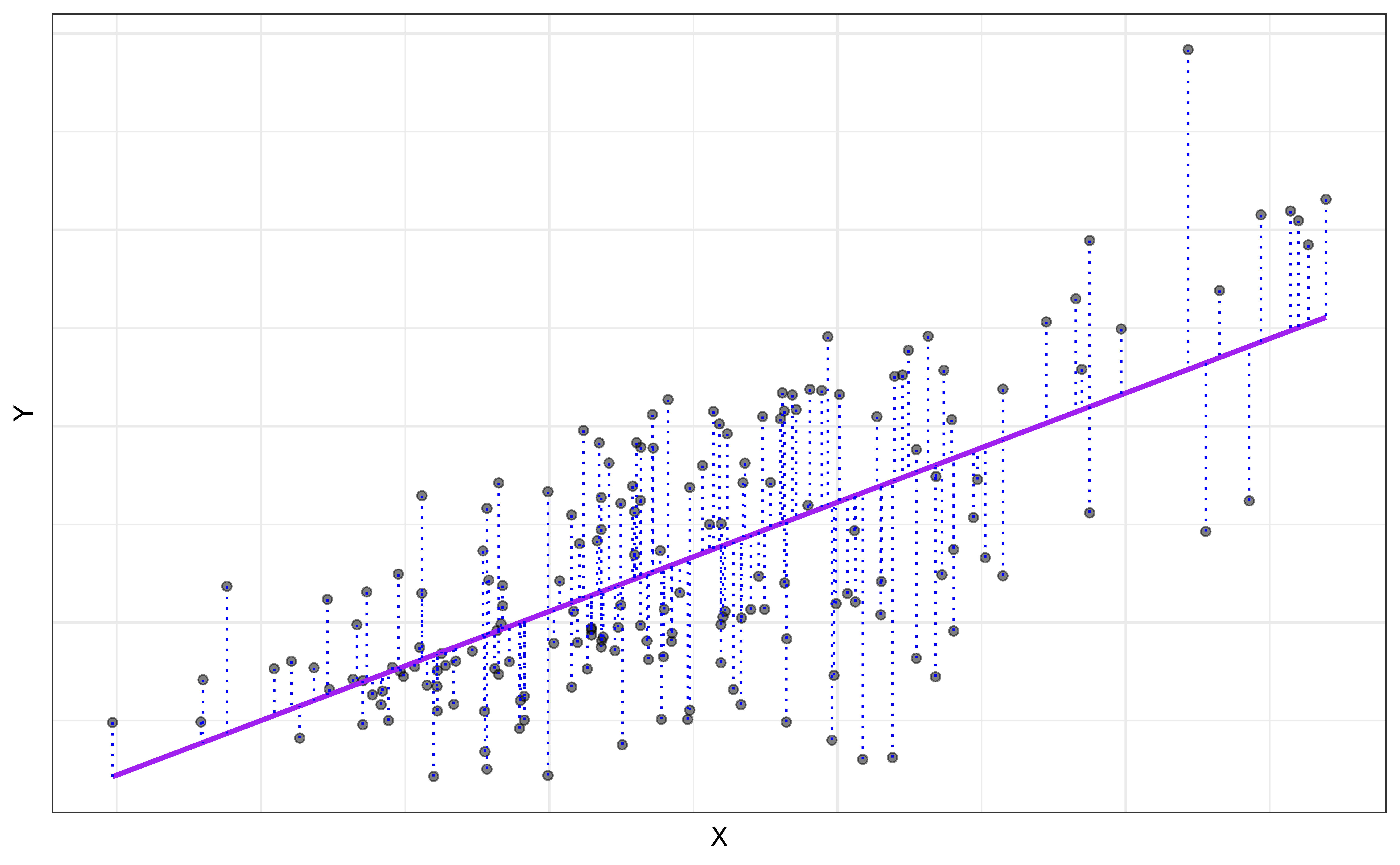
Simple linear regression (SLR)
SLR: Statistical model
- Simple linear regression: model to describe the relationship between \(Y\) and \(X\) where:
- \(Y\) is a quantitative/numerical response
- \(X\) is a single quantitative predictor
- \[\Large{Y = \mathbf{\beta_0 + \beta_1 X} + \epsilon}\]
- \(\beta_1\): True slope of the relationship between \(X\) and \(Y\)
- \(\beta_0\): True intercept of the relationship between \(X\) and \(Y\)
- \(\epsilon\): Error
SLR: Regression equation
\[\Large{\hat{Y} = \hat{\beta}_0 + \hat{\beta}_1 X}\]
- \(\hat{\beta}_1\): Estimated slope of the relationship between \(X\) and \(Y\)
- \(\hat{\beta}_0\): Estimated intercept of the relationship between \(X\) and \(Y\)
- \(\hat{Y}\): Predicted value of \(Y\) for a given \(X\)
- No error term!
Choosing values for \(\hat{\beta}_1\) and \(\hat{\beta}_0\)
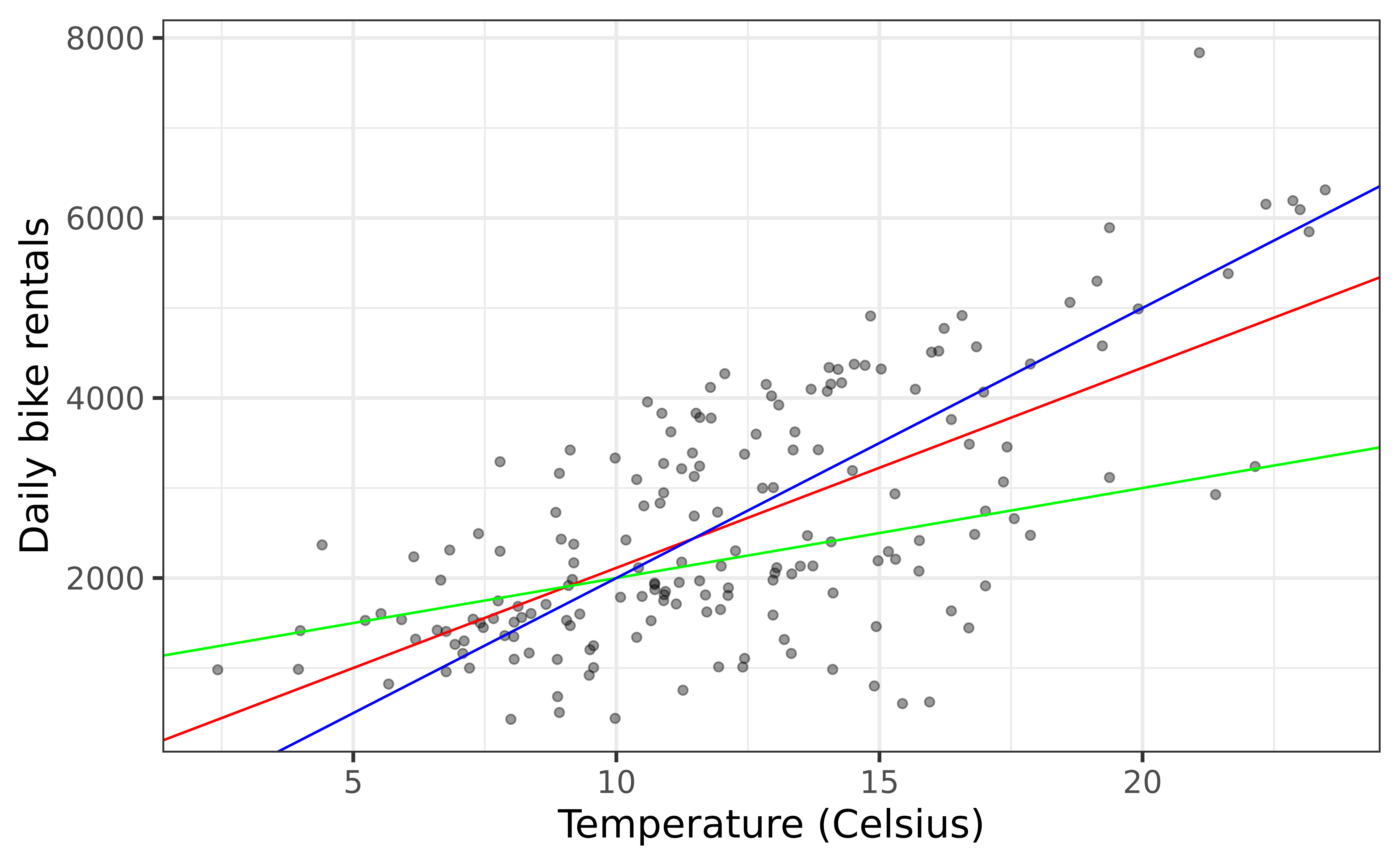
Residuals
`geom_smooth()` using formula = 'y ~ x'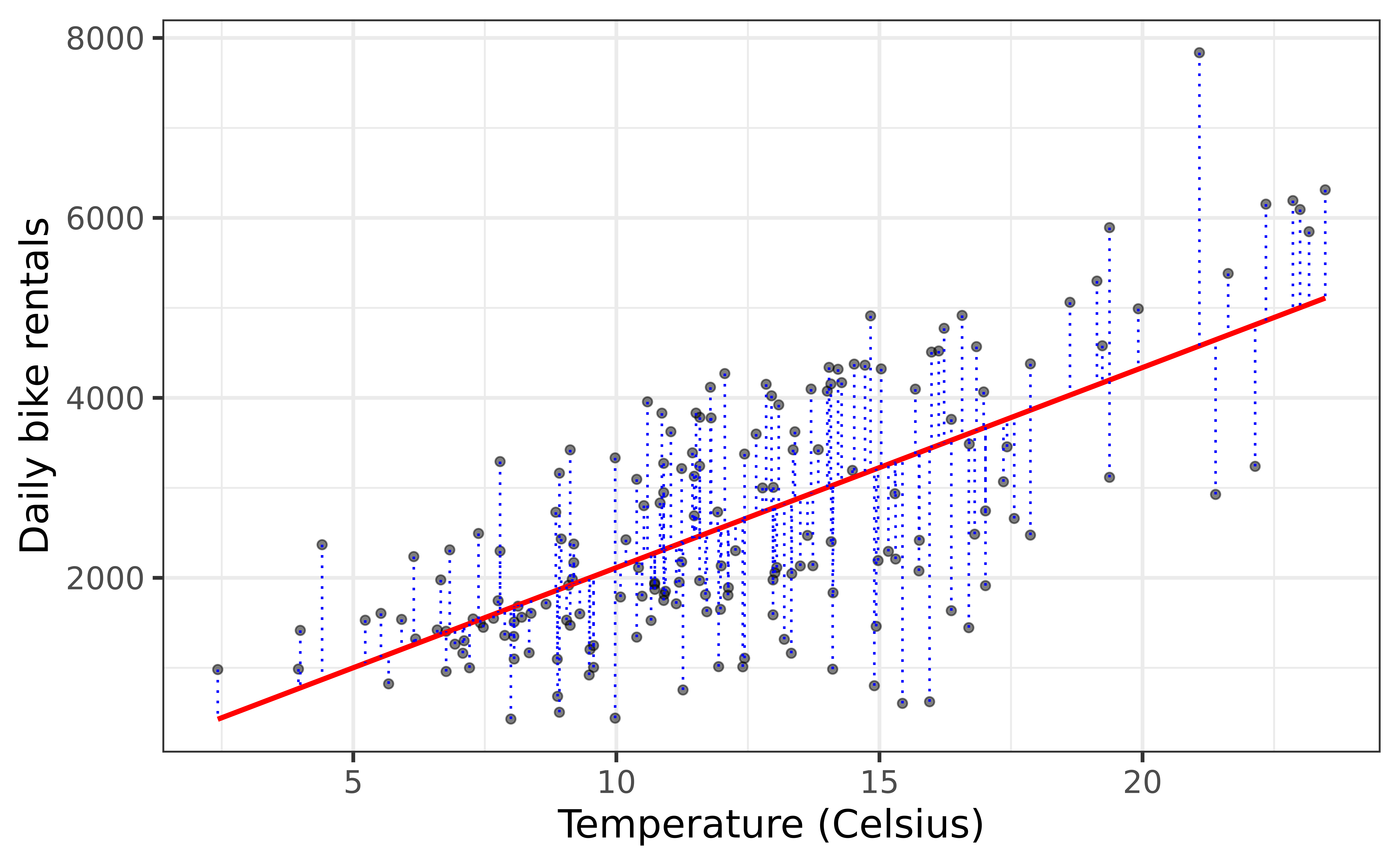
\[\text{residual} = \text{observed} - \text{predicted} = y_i - \hat{y}_i\]
Least squares line
- Residual for the \(i^{th}\) observation:
\[e_i = \text{observed} - \text{predicted} = y_i - \hat{y}_i\]
- Sum of squared residuals:
\[e^2_1 + e^2_2 + \dots + e^2_n\]
- Least squares line is the one that minimizes the sum of squared residuals
Recap
- Simple linear regression (SLR) describes the relationship between a quantitative predictor (\(X\)) and response (\(Y\)).
- The regression equation: \(\hat{Y} = \hat{\beta}_0 + \hat{\beta}_1 X\)
- \(\hat{\beta}_1\) (slope): estimated change in \(Y\) for each unit increase in \(X\)
- \(\hat{\beta}_0\) (intercept): estimated value of \(Y\) when \(X = 0\)
- Residuals: difference between observed and predicted values (\(e_i = y_i - \hat{y}_i\))
- Least squares method chooses coefficients to minimize the sum of squared residuals
- SLR can be used for prediction and inference
